K Index Calculation#
Show code cell content
# Install pooch (not currently in VRE)
import sys
!{sys.executable} -m pip install pooch

import datetime as dt
import numpy as np
import pandas as pd
import matplotlib.pyplot as plt
import pooch
from viresclient import SwarmRequest
import ipywidgets as widgets

from warnings import filterwarnings
filterwarnings(action="ignore")

# Data dependencies (pooch caches this in ~/.cache/pooch/)
esk_k_ind_file = pooch.retrieve(
    "https://raw.githubusercontent.com/MagneticEarth/IAGA_SummerSchool2019/master/data/external/k_inds/esk/2003.esk",
    known_hash="233246e167a212cd1afa33ff2fe130fbc308cd2ae7971c6c2afcd363c9775c18"
)
Collecting pooch
  Downloading pooch-1.8.2-py3-none-any.whl.metadata (10 kB)
Requirement already satisfied: platformdirs>=2.5.0 in /opt/conda/lib/python3.11/site-packages (from pooch) (4.0.0)
Requirement already satisfied: packaging>=20.0 in /opt/conda/lib/python3.11/site-packages (from pooch) (23.2)
Requirement already satisfied: requests>=2.19.0 in /opt/conda/lib/python3.11/site-packages (from pooch) (2.31.0)
Requirement already satisfied: charset-normalizer<4,>=2 in /opt/conda/lib/python3.11/site-packages (from requests>=2.19.0->pooch) (3.3.2)
Requirement already satisfied: idna<4,>=2.5 in /opt/conda/lib/python3.11/site-packages (from requests>=2.19.0->pooch) (3.6)
Requirement already satisfied: urllib3<3,>=1.21.1 in /opt/conda/lib/python3.11/site-packages (from requests>=2.19.0->pooch) (2.1.0)
Requirement already satisfied: certifi>=2017.4.17 in /opt/conda/lib/python3.11/site-packages (from requests>=2.19.0->pooch) (2024.12.14)
Downloading pooch-1.8.2-py3-none-any.whl (64 kB)
Installing collected packages: pooch
Successfully installed pooch-1.8.2
WARNING: Running pip as the 'root' user can result in broken permissions and conflicting behaviour with the system package manager, possibly rendering your system unusable. It is recommended to use a virtual environment instead: https://pip.pypa.io/warnings/venv. Use the --root-user-action option if you know what you are doing and want to suppress this warning.
[notice] A new release of pip is available: 25.1 -> 25.1.1
[notice] To update, run: pip install --upgrade pip
Downloading data from 'https://raw.githubusercontent.com/MagneticEarth/IAGA_SummerSchool2019/master/data/external/k_inds/esk/2003.esk' to file '/home/jovyan/.cache/pooch/cb259464aff5d2a782ba1ab3ddc07f1d-2003.esk'.
Calculating K-indices for a single observatory#
The K-index is a local geomagnetic activity index devised by Julius Bartels in 1938 to give a simple measure of the degree of geomagnetic disturbance during each 3-hour (UT) interval seen at a single magnetic observatory. Data from the observatory magnetometers are used to assign a number in the range 0-9 to each 3-hour interval, with K=0 indicating very little geomagnetic activity and K=9 representing an extreme geomagnetic storm. The K-index was introduced at the time of photographic recording, when magnetograms recorded variations in the horizontal geomagnetic field elements declination (D) and horizontal intensity (H), and in the vertical intensity (Z).
To derive a K-index an observer would fit, by eye, a ‘solar regular variation’ (
The conversion from range in nanoteslas to index is quasi-logarithmic. The conversion table varies with latitude in an attempt to normalise the K-index distribution for observatories at different latitudes. The table for Eskdalemuir is shown below.
K |
0 |
1 |
2 |
3 |
4 |
5 |
6 |
7 |
8 |
9 |
|---|---|---|---|---|---|---|---|---|---|---|
Lower bound (nT) |
0 |
8 |
15 |
30 |
60 |
105 |
180 |
300 |
500 |
750 |
This means that, for instance, K=2 if the measured range is in the interval [15, 30) nT.
There was a long debate in IAGA Division V about algorithms that could adequately reproduce the K-indices that an experienced observer would assign. The algorithms and code approved by IAGA are available at the International Service for Geomagnetic Indices: http://isgi.unistra.fr/softwares.php.
Example#
In the following cells, we illustrate a possible approach. We assume the so-called regular daily variation
For some days this simple approach to estimating
We then attempt to calculate K-indices for the day chosen by computing the Fourier series up the the number of harmonics selected by subtracting the synthetic harmonic signal from the data, then calculating 3-hr ranges and converting these into the corresponding K-index. The functions to do are also included in the following cell.
Show code cell source
def fourier(v, nhar):
    npts    = len(v)
    f       = 2.0/npts
    t       = np.linspace(0, npts, npts, endpoint=False)*2*np.pi/npts
    vmn     = np.mean(v)
    v       = v - vmn
    cofs    = [0]*(nhar+1)
    cofs[0] = (vmn,0)
    for i in range(1,nhar+1):
        c, s    = np.cos(i*t), np.sin(i*t)
        cofs[i] = (np.dot(v,c)*f, np.dot(v,s)*f)
    return (cofs)

def fourier_synth(cofs, npts):
    nt  = len(cofs)
    syn = np.zeros(npts)
    t  = np.linspace(0, npts, npts, endpoint=False)*2*np.pi/npts
    for n in range(1, nt):
        for j in range(npts):
            syn[j] += cofs[n][0]*np.cos(n*t[j]) + cofs[n][1]*np.sin(n*t[j])
    return (syn)

# Define K-index conversion table for ESK
K_conversions = {
    f"K{level}": level_bin
    for level, level_bin in enumerate(
        (0, 8, 15, 30, 60, 105, 180, 300, 500, 750)
    )
}
# Define reverse mapping
nT_to_K = {v: k for k, v in K_conversions.items()}

def K_calc(d, synd, Kb=K_conversions):
    tmp = np.ptp((d-synd).reshape(8,180), axis=1)
    return(list(np.digitize(tmp, bins=list(Kb.values()), right=False)-1))

def load_official_K(filepath=esk_k_ind_file):
    df = pd.read_csv(filepath, skiprows=0, header=None, delim_whitespace=True,
                     parse_dates=[[2,1,0]], index_col=0)
    df = df.drop(3, axis=1)
    df.index.name='Date'
    df.columns = ['00','03','06','09','12','15','18','21']
    return(df)

def load_ESK_2003():
    request = SwarmRequest()
    request.set_collection(f"SW_OPER_AUX_OBSM2_:ESK", verbose=False)
    request.set_products(measurements=["B_NEC", "IAGA_code"])
    data = request.get_between(
        dt.datetime(2003, 1, 1),
        dt.datetime(2004, 1, 1),
    )
    df = data.as_dataframe(expand=True)
    df = df.rename(columns={f"B_NEC_{i}": j for i, j in zip("NEC", "XYZ")})
    return df
First, load in (X, Y, Z) one-minute data from Eskdalemuir for 2003 into a pandas dataframe.
df_obs = load_ESK_2003()
df_obs.head()
| Radius | Longitude | Latitude | IAGA_code | X | Y | Z | |
|---|---|---|---|---|---|---|---|
| Timestamp | |||||||
| 2003-01-01 00:00:00 | 6.363967e+06 | 356.8 | 55.119672 | ESK | 17196.514832 | -1473.2 | 46252.152020 |
| 2003-01-01 00:01:00 | 6.363967e+06 | 356.8 | 55.119672 | ESK | 17196.014835 | -1473.4 | 46252.150446 |
| 2003-01-01 00:02:00 | 6.363967e+06 | 356.8 | 55.119672 | ESK | 17196.514832 | -1473.4 | 46252.152020 |
| 2003-01-01 00:03:00 | 6.363967e+06 | 356.8 | 55.119672 | ESK | 17196.715461 | -1473.8 | 46251.952650 |
| 2003-01-01 00:04:00 | 6.363967e+06 | 356.8 | 55.119672 | ESK | 17197.115459 | -1473.7 | 46251.953909 |
Load the official K index data (available from http://www.geomag.bgs.ac.uk/data_service/data/magnetic_indices/k_indices) to compare with later.
df_K_official = load_official_K()
df_K_official.head()
| 00 | 03 | 06 | 09 | 12 | 15 | 18 | 21 | |
|---|---|---|---|---|---|---|---|---|
| Date | ||||||||
| 2003-01-01 | 1 | 2 | 2 | 1 | 1 | 1 | 2 | 3 |
| 2003-01-02 | 2 | 0 | 0 | 1 | 1 | 1 | 2 | 2 |
| 2003-01-03 | 2 | 0 | 1 | 1 | 3 | 5 | 4 | 4 |
| 2003-01-04 | 4 | 4 | 2 | 2 | 2 | 2 | 3 | 3 |
| 2003-01-05 | 1 | 1 | 1 | 1 | 2 | 2 | 2 | 3 |
Evaluate K indices for a given day:
For each of
Perform a Fourier analysis on the data to find the regular daily variation,
Over each 3-hour interval, find the maximum differences from
Convert from nT to
Pick the greater of
Show code cell source
def analyse_day(day=dt.date(2003, 1, 1), n_harmonics=3, df=df_obs, df_K_official=df_K_official):
    """Generate figure illustrating the K index calculation for a given day"""
    # Select given day
    _df = df.loc[day.isoformat()]
    _df_K = df_K_official.loc[day.isoformat()]
    # Select X & Y data and remove daily mean
    x = (_df["X"] - _df["X"].mean()).values
    y = (_df["Y"] - _df["Y"].mean()).values
    # Perform Fourier analysis of X & Y separately
    xcofs = fourier(x, n_harmonics)
    synx  = fourier_synth(xcofs, len(x))
    ycofs = fourier(y, n_harmonics)
    syny  = fourier_synth(ycofs, len(y))

    # Build plot
    t = np.linspace(0, 1440, 1440, endpoint=False)/60
    fig, axes = plt.subplots(2, 1, figsize=(15, 10), sharex=True)
    # Plot X & Y data with approximated variation
    axes[0].plot(t, x, color="tab:blue", alpha=0.5)
    axes[0].plot(t, synx, color="tab:blue", label="X")
    axes[0].plot(t, y, color="tab:red", alpha=0.5)
    axes[0].plot(t, syny, color="tab:red", label="Y")
    # Plot the differences
    axes[1].plot(t, (x-synx), color="tab:blue")
    axes[1].plot(t, (y-syny), color="tab:red")

    # Find and plot min/max bounds over 3-hourly intervals
    minX = np.min((x-synx).reshape(8, 180), axis=1)
    maxX = np.max((x-synx).reshape(8, 180), axis=1)
    minY = np.min((y-syny).reshape(8, 180), axis=1)
    maxY = np.max((y-syny).reshape(8, 180), axis=1)
    t_3hours = np.linspace(0, 1440, 9, endpoint=True)/60
    axes[1].fill_between(t_3hours, list(minX)+[0], list(maxX)+[0], step="post", color="tab:blue", alpha=0.5)
    axes[1].fill_between(t_3hours, list(minY)+[0], list(maxY)+[0], step="post", color="tab:red", alpha=0.5)

    # Determine K index from each of X & Y
    K_X = np.digitize((maxX-minX), bins=list(K_conversions.values()), right=False) - 1
    K_Y = np.digitize((maxY-minY), bins=list(K_conversions.values()), right=False) - 1
    for i, (K_X_i, K_Y_i) in enumerate(zip(K_X, K_Y)):
        # Display determined K from X & Y
        px = i*3
        py = axes[1].get_ylim()[1]
        axes[1].annotate(
            f"K(X): {K_X_i}", (px, py), xytext=(30, 18),
            textcoords="offset pixels", color="tab:blue", size=12,
        )
        axes[1].annotate(
            f"K(Y): {K_Y_i}", (px, py), xytext=(30, 3),
            textcoords="offset pixels", color="tab:red", size=12,
        )
        # Display comparison with the official K index
        K_ours = max(K_X_i, K_Y_i)
        K_official = _df_K[i]
        axes[1].annotate(
            f"{K_ours}\n{K_official}",
            (i*3, axes[1].get_ylim()[0]), xytext=(40, -70), textcoords="offset pixels"
        )
    axes[1].annotate(
        f"Determined K:\nOfficial K:",
        (0, axes[1].get_ylim()[0]), xytext=(-80, -70), textcoords="offset pixels"
    )

    # Finalise figure
    for ax in axes:
        ax.grid()
        ax.xaxis.set_ticks(np.arange(0, 27, 3))
    axes[1].set_ylabel("Residuals [nT]")
    axes[1].set_xlabel("UT [hour]")
    axes[0].set_ylabel("[nT]")
    axes[0].legend(loc="upper right")
    fig.suptitle(f"ESK: {day.isoformat()}", y=0.9)

    return fig, axes

def make_widgets_K_index_calc():
    day = widgets.SelectionSlider(
        options=[t.date() for t in pd.date_range(dt.date(2003, 1, 1), dt.date(2003, 12, 31))],
        description="Select day:", layout=widgets.Layout(width='700px')
    )
#     day = widgets.DatePicker(value=dt.date(2003, 1, 1), description="Select day:")
    n_harmonics = widgets.SelectionSlider(options=range(1, 11), value=3, description="# harmonics:")
    return widgets.VBox(
        [day,
         n_harmonics,
         widgets.interactive_output(
             analyse_day,
             {"day": day, "n_harmonics": n_harmonics}
         )],
    )

make_widgets_K_index_calc()
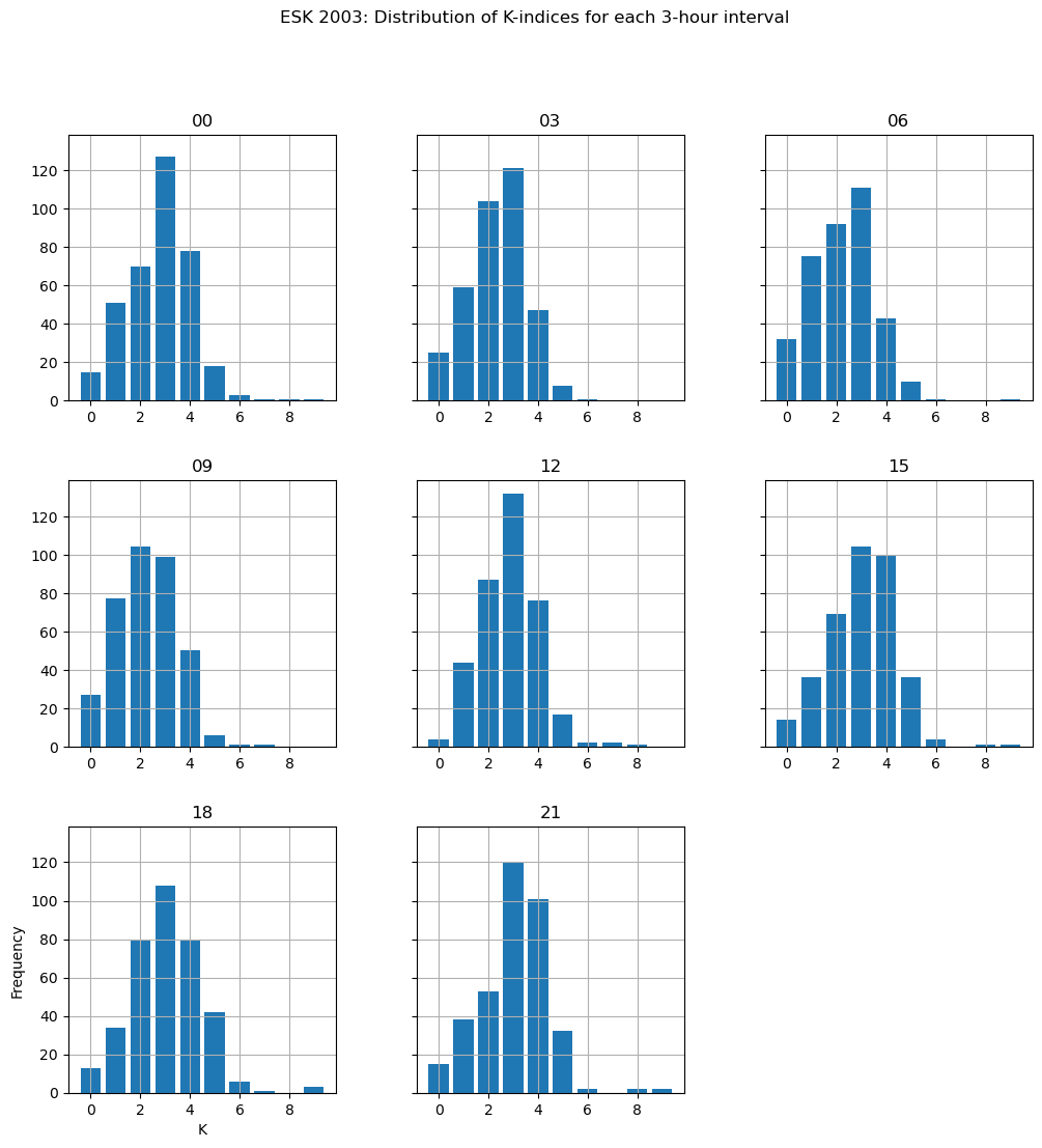
Statistics of the K index#
We will use the official K index from ESK to probe some statistics through the year 2003.
Histograms of the K indices for each 3-hour period:
axes = df_K_official.hist(
    figsize=(12, 12), bins=range(11), sharey=True, align="left", rwidth=0.8,
)
plt.suptitle('ESK 2003: Distribution of K-indices for each 3-hour interval')
axes[-1, 0].set_ylabel("Frequency")
axes[-1, 0].set_xlabel("K");
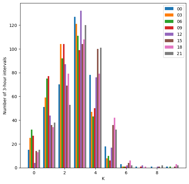
… plotted side by side:
plt.figure(figsize=(7,7))
plt.hist(df_K_official.values, bins=range(11), align='left')
plt.legend(df_K_official.columns)
plt.ylabel('Number of 3-hour intervals')
plt.xlabel('K');
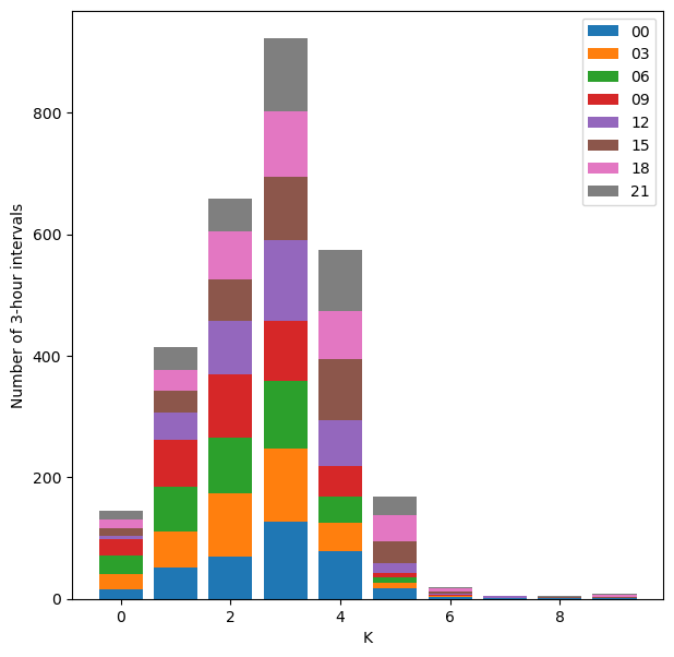
… and stacked together:
plt.figure(figsize=(7,7))
plt.hist(df_K_official.values, bins=range(11), stacked=True, align='left', rwidth=0.8)
plt.legend(df_K_official.columns)
plt.ylabel('Number of 3-hour intervals')
plt.xlabel('K');
We also compute a daily sum of the K-indices for the 2003 file, and list days with high and low summed values. Note that this summation is not really appropriate because the K-index is quasi-logarithmic, however, this is a common simple measure of quiet and disturbed days. (These might be interesting days for you to look at.)
df_K_official['Ksum'] = df_K_official.sum(axis=1)
Ksort = df_K_official.sort_values('Ksum')
print('Quiet days: \n\n', Ksort.head(10), '\n\n')
print('Disturbed days: \n\n', Ksort.tail(10))
Quiet days:

             00  03  06  09  12  15  18  21  Ksum
Date
2003-10-11   1   0   0   0   1   0   0   0     2
2003-12-19   0   0   0   0   1   0   0   1     2
2003-12-18   1   1   0   0   1   0   0   0     3
2003-03-25   0   1   1   0   1   1   1   0     5
2003-12-25   1   0   0   0   2   1   0   1     5
2003-01-08   2   0   1   0   1   0   1   0     5
2003-01-09   0   0   0   0   0   1   2   2     5
2003-07-08   0   0   0   0   2   2   1   0     5
2003-10-12   0   0   0   1   1   0   2   2     6
2003-01-16   1   0   0   1   2   0   1   1     6


Disturbed days:

             00  03  06  09  12  15  18  21  Ksum
Date
2003-09-17   4   5   4   4   5   5   4   5    36
2003-11-11   5   4   5   4   4   5   5   4    36
2003-02-02   5   4   4   4   4   6   5   5    37
2003-05-30   7   5   3   3   4   6   5   5    38
2003-05-29   3   3   3   2   6   6   7   8    38
2003-08-18   5   5   5   5   6   6   6   5    43
2003-11-20   1   3   5   4   7   9   9   8    46
2003-10-31   9   6   5   6   7   5   4   4    46
2003-10-30   8   5   4   4   5   5   9   9    49
2003-10-29   4   3   9   7   8   8   9   9    57
Note on the Fast Fourier Transform#
In the examples above we computed Fourier coefficients in the ‘traditional’ way, so that if
where
With
where the sampling interval
The fast Fourier transform (FFT) offers a computationally efficient means of finding the Fourier coefficients. The conventions for the FFT and its inverse (IFFT) vary from package to package. In the scipy.fftpack package, the FFT of a sequence
with the inverse defined as,
(The scipy documentation is perhaps a little confusing here because it explains the order of the
The interpretation is that if
and so we expect the relationship to the digitised Fourier series coefficients returned by the function fourier defined above to be,
The following shows the equivalence between the conventional Fourier series approach and the FFT.
from scipy.fftpack import fft

# Compute the fourier series as before
_df = df_obs.loc["2003-01-01"]
x = (_df["X"] - _df["X"].mean()).values
xcofs = fourier(x, 3)
# Compute using scipy FFT
npts = len(x)
xfft = fft(x)

# Compare results for the 24-hour component
k    = 1
print('Fourier coefficients: \n', f'A1 = {xcofs[1][0]} \n', f'B1 = {xcofs[1][1]} \n')
print('scipy FFT outputs: \n', f'a1 = {np.real(xfft[k]+xfft[npts-k])/npts} \n', \
      f'b1 = {-np.imag(xfft[k]-xfft[npts-k])/npts} \n')
Fourier coefficients:
 A1 = 1.9181527666779157
 B1 = 7.8492766783913055

scipy FFT outputs:
 a1 = 1.9181527666779157
 b1 = 7.849276678391305
References#
Menvielle, M. et al. (1995) ‘Computer production of K indices: review and comparison of methods’, Geophysical Journal International. Oxford University Press, 123(3), pp. 866–886. doi: 10.1111/j.1365-246X.1995.tb06895.x.