Spherical Harmonic Models 2#
# Import notebook dependencies
import sys
import matplotlib.pyplot as plt
import numpy as np
import pandas as pd

from src import sha, lsfile, cfile, IGRF13_FILE
A more tangible example of modelling using spherical harmonics#
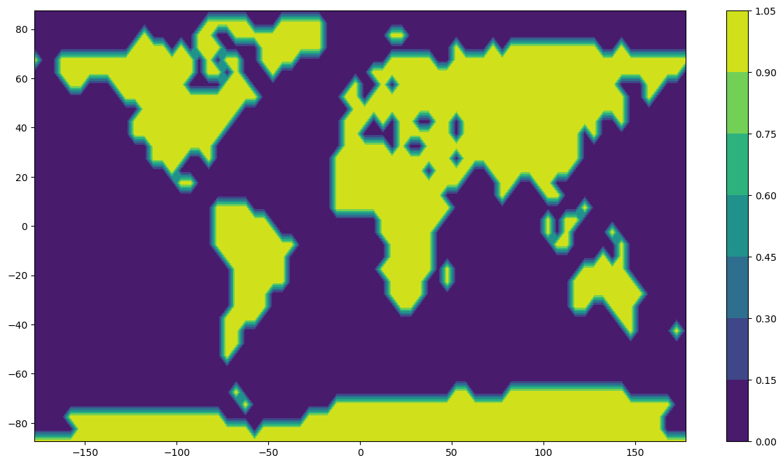
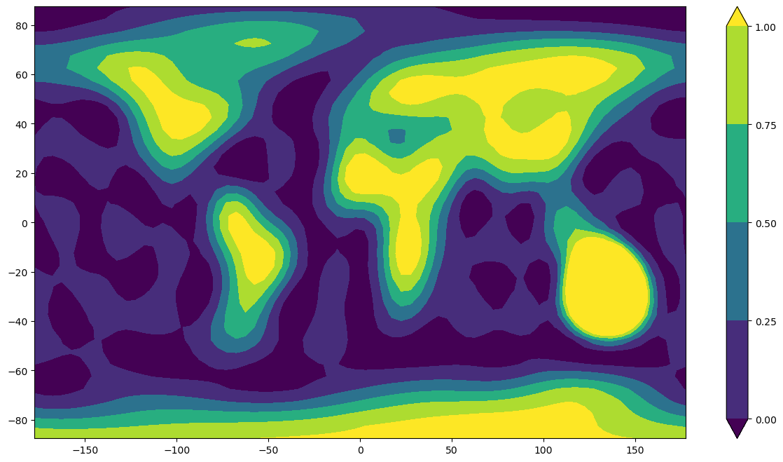
In this notebook we compute spherical harmonic models from an input data set representing a very simple world map with land encoded as 1 and water as 0 (so the data takes the values 0 and 1 only). We investigate the ability of models with different choices of maximum spherical harmonic degree to represent the data.
# Load the data
lsdata = np.genfromtxt(lsfile, delimiter=',')

x = lsdata[:,0].reshape(36, 72)
y = lsdata[:,1].reshape(36,72)
z = lsdata[:,2].reshape(36,72)

# Plot them
plt.rcParams['figure.figsize'] = [15, 8]
plt.contourf(x,y,z)
plt.colorbar()
plt.show()
>> USER INPUT HERE: Set the maximum spherical harmonic degree of the analysis
nmax = 10 # Max degree
# These functions are used for the spherical harmonic analysis and synthesis steps
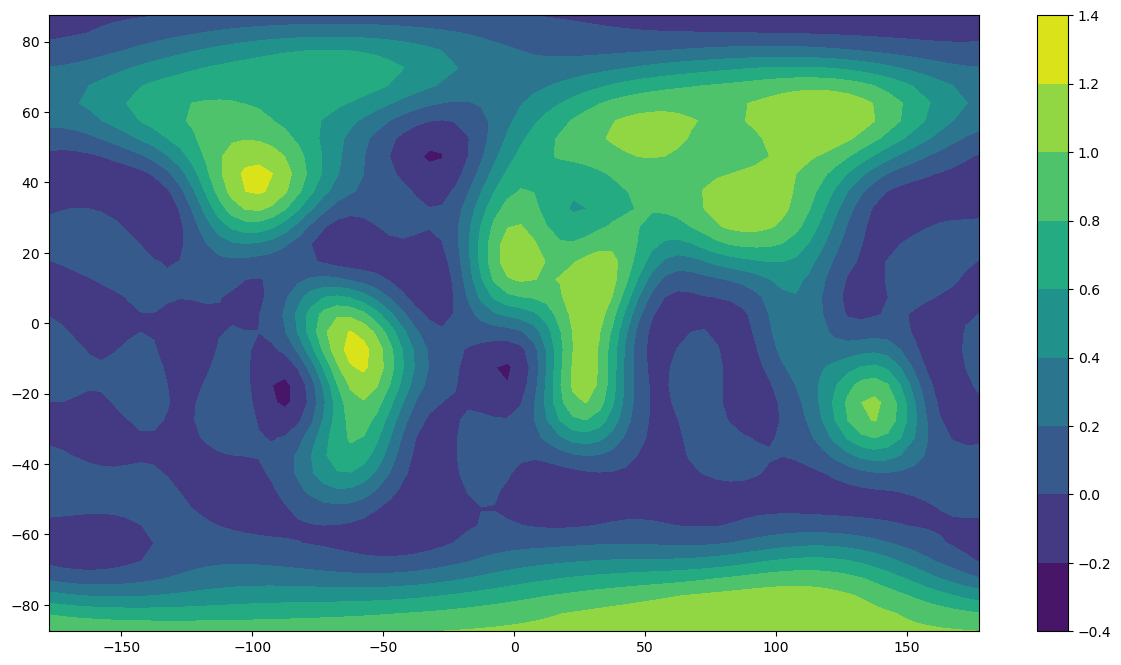
# Firstly compute a spherical harmonic model of degree and order nmax using the input data as plotted above
def sh_analysis(lsdata, nmax):
npar = (nmax+1)*(nmax+1)
ndat = len(lsdata)
lhs = np.zeros(npar*ndat).reshape(ndat,npar)
rhs = np.zeros(ndat)
line = np.zeros(npar)
ic = -1
for i in range(ndat):
th = 90 - lsdata[i][1]
ph = lsdata[i][0]
rhs[i] = lsdata[i][2]
cmphi, smphi = sha.csmphi(nmax,ph)
pnm = sha.pnm_calc(nmax, th)
for n in range(nmax+1):
igx = sha.gnmindex(n,0)
ipx = sha.pnmindex(n,0)
line[igx] = pnm[ipx]
for m in range(1,n+1):
igx = sha.gnmindex(n,m)
ihx = sha.hnmindex(n,m)
ipx = sha.pnmindex(n,m)
line[igx] = pnm[ipx]*cmphi[m]
line[ihx] = pnm[ipx]*smphi[m]
lhs[i,:] = line
shmod = np.linalg.lstsq(lhs, rhs.reshape(len(lsdata),1), rcond=None)
return(shmod)
# Now use the model to synthesise values on a 5 degree grid in latitude and longitude
def sh_synthesis(shcofs, nmax):
newdata =np.zeros(72*36*3).reshape(2592,3)
ic = 0
for ilat in range(36):
delta = 5*ilat+2.5
lat = 90 - delta
for iclt in range(72):
corr = 5*iclt+2.5
long = -180+corr
colat = 90-lat
cmphi, smphi = sha.csmphi(nmax,long)
vals = np.dot(sha.gh_phi(shcofs, nmax, cmphi, smphi), sha.pnm_calc(nmax, colat))
newdata[ic,0]=long
newdata[ic,1]=lat
newdata[ic,2]=vals
ic += 1
return(newdata)
# Obtain the spherical harmonic coefficients
shmod = sh_analysis(lsdata=lsdata, nmax=nmax)

# Read the model coefficients
shcofs = shmod[0]

# Synthesise the model coefficients on a 5 degree grid
newdata = sh_synthesis(shcofs=shcofs, nmax=nmax)
# Reshape for plotting purposes
x = newdata[:,0].reshape(36, 72)
y = newdata[:,1].reshape(36,72)
z = newdata[:,2].reshape(36,72)

# Plot the results
plt.rcParams['figure.figsize'] = [15, 8]
levels = [-1.5, -0.75, 0, 0.25, 0.5, 0.75, 2.]
plt.contourf(x,y,z)
plt.colorbar()
plt.show()
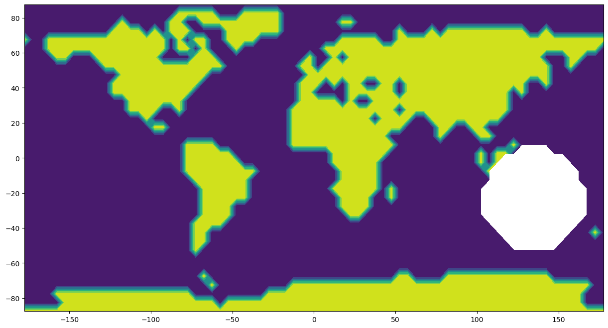
Spherical harmonic models with data gaps#
What happens if the data set is incomplete? In this section, you can experiment by removing data within a spherical cap of specified radius and pole position.
def greatcircle(th1, ph1, th2, ph2):
    th1 = np.deg2rad(th1)
    th2 = np.deg2rad(th2)
    dph = np.deg2rad(dlong(ph1,ph2))

  # Apply the cosine rule of spherical trigonometry
    dth = np.arccos(np.cos(th1)*np.cos(th2) + \
              np.sin(th1)*np.sin(th2)*np.cos(dph))
    return(dth)

def dlong (ph1, ph2):
    ph1 = np.sign(ph1)*abs(ph1)%360   # These lines return a number in the
    ph2 = np.sign(ph2)*abs(ph2)%360   # range -360 to 360
    if(ph1 < 0): ph1 = ph1 + 360      # Put the results in the range 0-360
    if(ph2 < 0): ph2 = ph2 + 360
    dph = max(ph1,ph2) - min(ph1,ph2) # So the answer is positive and in the
                                      # range 0-360
    if(dph > 180): dph = 360-dph      # So the 'short route' is returned
    return(dph)

def gh_phi(gh, nmax, cp, sp):
    rx = np.zeros(nmax*(nmax+3)//2+1)
    igx=-1
    igh=-1
    for i in range(nmax+1):
        igx += 1
        igh += 1
        rx[igx]= gh[igh]
        for j in range(1,i+1):
            igh += 2
            igx += 1
            rx[igx] = (gh[igh-1]*cp[j] + gh[igh]*sp[j])
    return(rx)
>> USER INPUT HERE: Set the location and size of the data gap
Enter the pole colatitude and longitude in degrees and the radius in km
# Remove a section of data centered on colat0, long0 and radius='radius':
colat0  = 113
long0   = 135
radius  = 3000
lsdata_gap = lsdata.copy()
for row in range(len(lsdata_gap)):
    colat = 90 - lsdata_gap[row,1]
    long  = lsdata_gap[row,0]
    if greatcircle(colat, long, colat0, long0) < radius/6371.2:
        lsdata_gap[row,2] = np.nan

print('Blanked out: ', np.count_nonzero(np.isnan(lsdata_gap)))

x_gap = lsdata_gap[:,0].reshape(36, 72)
y_gap = lsdata_gap[:,1].reshape(36,72)
z_gap = lsdata_gap[:,2].reshape(36,72)

# Plot the map with omitted data
plt.contourf(x_gap, y_gap, z_gap)
Blanked out: 104
<matplotlib.contour.QuadContourSet at 0x7f3aa4a6f710>
USER INPUT HERE: Set the maximum spherical harmonic degree of the analysis
nmax = 12 #Max degree
# Select the non-nan data
lsdata_gap = lsdata_gap[~np.isnan(lsdata_gap[:,2])]

# Obtain the spherical harmonic coefficients for the incomplete data set
shmod = sh_analysis(lsdata=lsdata_gap, nmax=nmax)

# Read the model coefficients
shcofs = shmod[0]

# Synthesise the model coefficients on a 5 degree grid
newdata = sh_synthesis(shcofs=shcofs, nmax=nmax)
# Reshape for plotting purposes
x_new = newdata[:,0].reshape(36, 72)
y_new = newdata[:,1].reshape(36,72)
z_new = newdata[:,2].reshape(36,72)
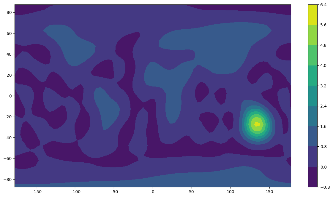
Print the maximum and minimum of the synthesised data. How do they compare to the original data, which was composed of only ones and zeroes? How do the max/min change as you vary the data gap size and the analysis resolution? Why? Try this with a larger gap, e.g. 5000 km.
print(np.min(z_new))
print(np.max(z_new))
-0.25531903688873575
5.853211492921363
# Plot the results with colour scale according to the data
plt.rcParams['figure.figsize'] = [15, 8]
plt.contourf(x_new, y_new, z_new)
plt.colorbar()
plt.show()
Now see what happens when we restrict the colour scale to values between 0 and 1 (so values <0 and >1 are compressed into opposite ends of the colour scale).
# Plot the results
plt.rcParams['figure.figsize'] = [15, 8]
levels = [0, 0.25, 0.5, 0.75, 1.]
plt.contourf(x_new, y_new, z_new, levels, extend='both')
plt.colorbar()
plt.show()
Making a spherical harmonic model of the geomagnetic field#
There is a file containing virtual observatory (VO) data calculated from the Swarm 3-satellite constellation in this repository. VOs use a local method to provide point estimates of the magnetic field at a specified time and fixed location at satellite altitude. This technique has various benefits, including:
Easier comparison between satellite (moving instrument) and ground observatory (fixed instrument) data, which is particularly useful when studying time changes of the magnetic field, e.g. geomagnetic jerks.
One can compute VOs on a regular spatial grid to mitigate the effects of uneven ground observatory coverage.
A brief summary of the method used to calculate each of these VO data points:
Swarm track data over four months are divided into 300 globally distributed equal area bins
Gross outliers (deviating over 500nT from the CHAOS-6-x7 internal field model) are removed
Only data from magnetically quiet, dark times are kept
Estimates of the core and crustal fields from CHAOS-6-x7 are subtracted from each datum to give the residuals
A local magnetic potential
Values of the residual magnetic field in spherical coordinates (
An estimate of the modelled core field at the VO calculation point is added back onto the residual field to give the total internal magnetic field value
In this section, we use VO data centred on 2015.0 to produce a degree 13 spherical harmonic model of the geomagnetic field and compare our (satellite data only) model to the IGRF (computed using both ground and satellite data) at 2015.0.
# Read in the VO data
cols  = ['Year','Colat','Long','Rad','Br','Bt', 'Bp']
bvals = pd.read_csv(cfile, sep='\s+', skiprows=0, header=None, index_col=0,
                    na_values=[99999.00,99999.00000], names=cols, comment='%')
bvals = bvals.dropna()
bvals['Bt']= -bvals['Bt']
bvals['Br']= -bvals['Br']
colnames=['Colat','Long','Rad','Bt','Bp', 'Br']
bvals=bvals.reindex(columns=colnames)
bvals.columns = ['Colat','Long','Rad','X','Y','Z']
print(bvals.info())
# Set the date to 2015.0 (this is the only common date between the VO data file and the IGRF coefficients file)
epoch = 2015.0
# Set the model resolution to 13 (the same as IGRF)
nmax = 13
<class 'pandas.core.frame.DataFrame'>
Index: 1444 entries, 2014.0 to 2018.0
Data columns (total 6 columns):
 #   Column  Non-Null Count  Dtype
---  ------  --------------  -----
 0   Colat   1444 non-null   float64
 1   Long    1444 non-null   float64
 2   Rad     1444 non-null   float64
 3   X       1444 non-null   float64
 4   Y       1444 non-null   float64
 5   Z       1444 non-null   float64
dtypes: float64(6)
memory usage: 79.0 KB
None
def geomagnetic_model(epoch, nmax, data, RREF=6371.2):
    # Select the data for that date
    colat =  np.array(data.loc[epoch]['Colat'])
    nx   = len(colat) # Number of data triples
    ndat = 3*nx    # Total number of data
    elong =  np.array(data.loc[epoch]['Long'])
    rad   =  np.array(data.loc[epoch]['Rad'])
    rhs   =  data.loc[epoch][['X', 'Y', 'Z']].values.reshape(ndat,1)
    npar = (nmax+1)*(nmax+1) # Number of model parameters
    nx   = len(colat) # Number of data triples
    ndat = 3*nx    # Total number of data
    print('Number of data triples selected =', nx)

    # Arrays for the equations of condition
    lhs  = np.zeros(npar*ndat).reshape(ndat,npar)
    linex = np.zeros(npar); liney = np.zeros(npar); linez = np.zeros(npar)

    iln = 0 # Row counter
    for i in range(nx): # Loop over data triplets (X, Y, Z)
        r  = rad[i]
        th = colat[i]; ph  = elong[i]
        rpow = sha.rad_powers(nmax, RREF, r)
        cmphi, smphi = sha.csmphi(nmax, ph)
        pnm, xnm, ynm, znm = sha.pxyznm_calc(nmax, th)

        for n in range(nmax+1): # m=0
            igx = sha.gnmindex(n,0) # Index for g(n,0) in gh conventional order
            ipx = sha.pnmindex(n,0) # Index for pnm(n,0) in array pnm
            rfc = rpow[n]
            linex[igx] =  xnm[ipx]*rfc
            liney[igx] =  0
            linez[igx] = znm[ipx]*rfc

            for m in range(1,n+1): # m>0
                igx = sha.gnmindex(n,m) # Index for g(n,m)
                ihx = igx + 1           # Index for h(n,m)
                ipx = sha.pnmindex(n,m) # Index for pnm(n,m)
                cpr = cmphi[m]*rfc
                spr = smphi[m]*rfc
                linex[igx] =  xnm[ipx]*cpr; linex[ihx] =  xnm[ipx]*spr
                liney[igx] =  ynm[ipx]*spr; liney[ihx] = -ynm[ipx]*cpr
                linez[igx] =  znm[ipx]*cpr; linez[ihx] =  znm[ipx]*spr

        lhs[iln,  :] = linex
        lhs[iln+1,:] = liney
        lhs[iln+2 :] = linez
        iln += 3

    shmod = np.linalg.lstsq(lhs, rhs, rcond=None) # Include the monopole
    # shmod = np.linalg.lstsq(lhs[:,1:], rhs, rcond=None) # Exclude the monopole
    gh = shmod[0]
    return(gh)
coeffs = geomagnetic_model(epoch=epoch, nmax=nmax, data=bvals)
Number of data triples selected = 299
Read in the IGRF coefficients for comparison
igrf13 = pd.read_csv(IGRF13_FILE, delim_whitespace=True, header=3)
igrf13.head()
| g/h | n | m | 1900.0 | 1905.0 | 1910.0 | 1915.0 | 1920.0 | 1925.0 | 1930.0 | ... | 1980.0 | 1985.0 | 1990.0 | 1995.0 | 2000.0 | 2005.0 | 2010.0 | 2015.0 | 2020.0 | 2020-25 | |
|---|---|---|---|---|---|---|---|---|---|---|---|---|---|---|---|---|---|---|---|---|---|
| 0 | g | 1 | 0 | -31543 | -31464 | -31354 | -31212 | -31060 | -30926 | -30805 | ... | -29992 | -29873 | -29775 | -29692 | -29619.4 | -29554.63 | -29496.57 | -29441.46 | -29404.8 | 5.7 |
| 1 | g | 1 | 1 | -2298 | -2298 | -2297 | -2306 | -2317 | -2318 | -2316 | ... | -1956 | -1905 | -1848 | -1784 | -1728.2 | -1669.05 | -1586.42 | -1501.77 | -1450.9 | 7.4 |
| 2 | h | 1 | 1 | 5922 | 5909 | 5898 | 5875 | 5845 | 5817 | 5808 | ... | 5604 | 5500 | 5406 | 5306 | 5186.1 | 5077.99 | 4944.26 | 4795.99 | 4652.5 | -25.9 |
| 3 | g | 2 | 0 | -677 | -728 | -769 | -802 | -839 | -893 | -951 | ... | -1997 | -2072 | -2131 | -2200 | -2267.7 | -2337.24 | -2396.06 | -2445.88 | -2499.6 | -11.0 |
| 4 | g | 2 | 1 | 2905 | 2928 | 2948 | 2956 | 2959 | 2969 | 2980 | ... | 3027 | 3044 | 3059 | 3070 | 3068.4 | 3047.69 | 3026.34 | 3012.20 | 2982.0 | -7.0 |
5 rows × 29 columns
# Select the 2015 IGRF coefficients
igrf = np.array(igrf13[str(epoch)])
# Insert a zero in place of the monopole coefficient (this term is NOT included in the IRGF, or any other field model)
igrf = np.insert(igrf, 0, 0)
Compare our model coefficients to IGRF13
print("VO only model \t   IGRF13")
for i in range(196):
    print("% 9.1f\t%9.1f" %(coeffs[i], igrf[i]))
VO only model 	   IGRF13
     -0.3	      0.0
 -29441.9	 -29441.5
  -1502.9	  -1501.8
   4784.9	   4796.0
  -2444.7	  -2445.9
   3012.8	   3012.2
  -2826.6	  -2845.4
   1676.4	   1676.3
   -640.9	   -642.2
   1351.9	   1350.3
  -2352.0	  -2352.3
   -135.5	   -115.3
   1225.7	   1225.8
    245.0	    245.0
    582.6	    581.7
   -538.8	   -538.7
    907.9	    907.4
    813.9	    813.7
    304.4	    283.5
    120.9	    120.5
   -189.0	   -188.4
   -335.3	   -334.9
    180.7	    180.9
     70.7	     70.4
   -329.0	   -329.2
   -233.0	   -232.9
    359.9	    360.1
     23.9	     47.0
    192.4	    192.3
    196.8	    197.0
   -141.0	   -140.9
   -119.1	   -119.1
   -157.5	   -157.4
     15.7	     16.0
      3.9	      4.3
    100.1	    100.1
     69.5	     69.5
     68.0	     67.6
      4.3	    -20.6
     72.9	     72.8
     33.5	     33.3
   -130.0	   -129.8
     58.9	     58.7
    -28.9	    -28.9
    -66.6	    -66.6
     13.2	     13.1
      7.3	      7.3
    -71.0	    -70.8
     62.4	     62.4
     81.4	     81.3
    -76.1	    -76.0
    -81.8	    -54.3
     -6.7	     -6.8
    -19.6	    -19.5
     51.7	     51.8
      5.6	      5.6
     15.1	     15.1
     24.5	     24.4
      9.4	      9.3
      3.3	      3.3
     -2.8	     -2.9
    -27.5	    -27.5
      6.6	      6.6
     -2.3	     -2.3
     24.2	     24.0
      9.1	      8.9
     39.4	     10.0
    -16.7	    -16.8
    -18.3	    -18.3
     -3.2	     -3.2
     13.2	     13.2
    -20.5	    -20.6
    -14.7	    -14.6
     13.3	     13.3
     16.2	     16.2
     11.8	     11.8
      5.7	      5.7
    -15.9	    -16.0
     -9.2	     -9.1
     -2.0	     -2.0
      2.2	      2.3
      5.4	      5.3
      8.7	      8.8
    -53.8	    -21.8
      3.0	      3.0
     10.7	     10.8
     -3.4	     -3.2
     11.8	     11.7
      0.7	      0.7
     -6.8	     -6.7
    -13.2	    -13.2
     -6.9	     -6.9
     -0.2	     -0.1
      7.7	      7.8
      8.7	      8.7
      1.1	      1.0
     -9.0	     -9.1
     -3.9	     -3.9
    -10.5	    -10.5
      8.4	      8.4
     -2.0	     -2.0
     -6.0	     -6.3
     37.6	      3.3
      0.2	      0.2
     -0.3	     -0.4
      0.5	      0.6
      4.5	      4.5
     -0.5	     -0.6
      4.4	      4.4
      1.7	      1.7
     -7.9	     -7.9
     -0.6	     -0.7
     -0.6	     -0.6
      2.2	      2.1
     -4.2	     -4.2
      2.4	      2.3
     -2.8	     -2.9
     -1.8	     -1.8
     -1.1	     -1.1
     -3.6	     -3.6
     -8.7	     -8.7
      3.0	      3.0
     -1.5	     -1.4
    -37.5	      0.0
     -2.3	     -2.3
      2.1	      2.1
      2.0	      2.1
     -0.6	     -0.6
     -0.8	     -0.8
     -1.0	     -1.1
      0.6	      0.6
      0.7	      0.8
     -0.8	     -0.7
     -0.3	     -0.2
      0.2	      0.1
     -2.1	     -2.1
      1.7	      1.7
     -1.4	     -1.4
     -0.2	     -0.2
     -2.5	     -2.6
      0.4	      0.4
     -2.0	     -2.0
      3.5	      3.5
     -2.3	     -2.3
     -2.1	     -2.1
      0.1	     -0.2
     38.8	     -1.1
      0.5	      0.5
      0.5	      0.4
      1.2	      1.2
      1.7	      1.8
     -0.9	     -0.9
     -2.2	     -2.2
      0.9	      0.8
      0.2	      0.3
      0.2	      0.1
      0.7	      0.7
      0.5	      0.5
     -0.1	     -0.1
     -0.3	     -0.4
      0.3	      0.3
     -0.5	     -0.4
      0.2	      0.2
      0.2	      0.2
     -0.9	     -0.9
     -0.9	     -0.9
     -0.2	     -0.2
      0.0	     -0.0
      0.7	      0.7
     -0.0	     -0.0
     -1.0	     -0.9
    -44.6	     -0.9
      0.4	      0.4
      0.4	      0.5
      0.6	      0.6
      1.6	      1.6
     -0.5	     -0.4
     -0.5	     -0.5
      1.0	      1.0
     -1.3	     -1.2
     -0.4	     -0.2
     -0.2	     -0.1
      0.9	      0.8
      0.4	      0.4
     -0.2	     -0.1
     -0.0	     -0.0
      0.4	      0.4
      0.5	      0.5
      0.0	      0.1
      0.5	      0.5
      0.5	      0.5
     -0.3	     -0.3
     -0.3	     -0.3
     -0.4	     -0.4
     -0.3	     -0.4
     -0.7	     -0.7
/tmp/ipykernel_4802/715981350.py:3: DeprecationWarning: Conversion of an array with ndim > 0 to a scalar is deprecated, and will error in future. Ensure you extract a single element from your array before performing this operation. (Deprecated NumPy 1.25.)
  print("% 9.1f\t%9.1f" %(coeffs[i], igrf[i]))
Exercise#
Above we took a simple approach and computed a model for 2015.0 uding VO data for 2015.0. Use VOs to produce a model at a time of your choice between 2014 and 2018 (other than 2015.0 as we did above) and compare your coefficients to the IGRF at that time. Hints: For dates other than yyyy.0, you will need to interpolate the IGRF coefficients.
Exercise#
Create a second spherical harmonic model based on ground observatory data only and compare it to your satellite data only model and to the IGRF. To do this, you can use observatory annual means as the input data, which we have supplied in the file oamjumpsapplied.dat in the external data directory. Hint: The mag module contains a function that will extract all annual mean values for all observatories in a given year.
# Install pooch (not currently in VRE)
import sys
!{sys.executable} -m pip install pooch
Requirement already satisfied: pooch in /opt/conda/lib/python3.11/site-packages (1.8.2)
Requirement already satisfied: platformdirs>=2.5.0 in /opt/conda/lib/python3.11/site-packages (from pooch) (4.0.0)
Requirement already satisfied: packaging>=20.0 in /opt/conda/lib/python3.11/site-packages (from pooch) (23.2)
Requirement already satisfied: requests>=2.19.0 in /opt/conda/lib/python3.11/site-packages (from pooch) (2.31.0)
Requirement already satisfied: charset-normalizer<4,>=2 in /opt/conda/lib/python3.11/site-packages (from requests>=2.19.0->pooch) (3.3.2)
Requirement already satisfied: idna<4,>=2.5 in /opt/conda/lib/python3.11/site-packages (from requests>=2.19.0->pooch) (3.6)
Requirement already satisfied: urllib3<3,>=1.21.1 in /opt/conda/lib/python3.11/site-packages (from requests>=2.19.0->pooch) (2.1.0)
Requirement already satisfied: certifi>=2017.4.17 in /opt/conda/lib/python3.11/site-packages (from requests>=2.19.0->pooch) (2024.12.14)
WARNING: Running pip as the 'root' user can result in broken permissions and conflicting behaviour with the system package manager, possibly rendering your system unusable. It is recommended to use a virtual environment instead: https://pip.pypa.io/warnings/venv. Use the --root-user-action option if you know what you are doing and want to suppress this warning.

[notice] A new release of pip is available: 25.1 -> 25.2
[notice] To update, run: pip install --upgrade pip
# Fetch the data and import the relevant function
import pooch

oamjumpsapplied = pooch.retrieve(
    "https://raw.githubusercontent.com/MagneticEarth/IAGA_SummerSchool2019/master/data/external/oamjumpsapplied.dat",
    known_hash="dee77ded79cb0d86e3366a550830cad9de741322212faf9a74f3d03cb6bdd872"
)

from src.mag import obs_ann_means_one_year
Downloading data from 'https://raw.githubusercontent.com/MagneticEarth/IAGA_SummerSchool2019/master/data/external/oamjumpsapplied.dat' to file '/home/jovyan/.cache/pooch/c1a0acda735b5c4d0b60def6e59ddb56-oamjumpsapplied.dat'.
input_data = obs_ann_means_one_year(2000, oamjumpsapplied)
input_data
| Code | Colat | Long | alt(m) | year | D | I | H | X | Y | Z | F | |
|---|---|---|---|---|---|---|---|---|---|---|---|---|
| 1 | ALE | 7.500 | 297.650 | 60 | 2000.5 | -67.510 | 86.448 | 3448 | 1319 | -3186 | 55553 | 55660 |
| 2 | NAL | 11.083 | 11.933 | 12 | 2000.5 | 0.332 | 82.317 | 7263 | 7263 | 42 | 53841 | 54329 |
| 3 | CCS | 12.283 | 104.283 | 10 | 2000.5 | 14.762 | 87.143 | 2929 | 2832 | 746 | 58709 | 58781 |
| 4 | THL | 12.517 | 290.833 | 57 | 2000.5 | -63.167 | 86.060 | 3877 | 1750 | -3460 | 56298 | 56431 |
| 5 | HRN | 13.000 | 15.550 | 15 | 2000.5 | 2.925 | 81.500 | 7996 | 7986 | 408 | 53504 | 54098 |
| ... | ... | ... | ... | ... | ... | ... | ... | ... | ... | ... | ... | ... |
| 196 | SYO | 159.000 | 39.583 | 0 | 2000.6 | -48.527 | -63.777 | 19168 | 12694 | -14362 | -38913 | 43378 |
| 197 | VNA | 160.650 | 351.750 | 40 | 2000.5 | -12.907 | -61.207 | 18977 | 18498 | -4239 | -34529 | 39400 |
| 198 | TNB | 164.683 | 164.117 | 28 | 2000.0 | 136.233 | -83.013 | 7829 | -5654 | 5415 | -63886 | 64364 |
| 199 | SBA | 167.850 | 166.783 | 10 | 2000.5 | 155.260 | -80.390 | 11212 | -10183 | 4692 | -66219 | 67161 |
| 200 | VOS | 168.450 | 106.867 | 3500 | 2000.5 | -120.678 | -76.992 | 13443 | -6859 | -11562 | -58192 | 59725 |
200 rows × 12 columns
Acknowledgements#
The land/sea data file was provided by John Stevenson (BGS). The VO data were computed by Magnus Hammer (DTU) and the file prepared by Will Brown (BGS).