Lorenz’s (1963) model: forward modelling

\[ \newcommand{\myd}{\mathrm{d}} \newcommand{\statev}{\mathbf{X}} \newcommand{\lrayleigh}{{\mathrm{r}}} \newcommand{\rayleigh}{{\mathrm{Ra}}} \newcommand{\pr}{\mathrm{Pr}} \newcommand{\adj}{T} \newcommand{\tstep}{\Delta t} \]

Introduction

A good understanding of the forward model is mandatory before any practice of data assimilation. The goal of this first notebook is to get familiar with the numerical model we are dealing with today. The model we are interested in is the famous model proposed by Edward Lorenz in 1963. This model is the canonical example of a set of coupled deterministic, nonlinear, ordinary differential equations (ode) able to exhibit chaotic behaviour. It is a simplified, 3-variable representation of atmospheric cellular convection, based on the earlier work of Saltzman (1962).

Its time evolution is governed by the following set of nondimensional equations

\[\begin{split} \begin{eqnarray} \frac{\myd X}{\myd t} &=& -\pr (X -Y), \label{eq:lorx}\\ \frac{\myd Y}{\myd t} &=& -XZ +\lrayleigh X -Y, \label{eq:lory}\\ \frac{\myd Z}{\myd t} &=& XY - bZ,\label{eq:lorz} \end{eqnarray} \end{split}\]

which has to be supplemented with a (column) vector of initial conditions

\[ \statev_0=\left[X(t=0),Y(t=0),Z(t=0) \right]^{\adj}. \]

The variable \(X\) is connected with the streamfunction describing atmospheric flow, while both variables \(Y\) and \(Z\) are connected with the temperature deviation responsible for convection. So the state of atmospheric quiescence (no convection) is described by \(\statev=[0,0,0]^\adj\).

Three nondimensional numbers define the parameter space:

• \(\pr\), the Prandtl number, which is the ratio of kinematic viscosity to thermal diffusivity

• \(\lrayleigh\), which is the ratio of the Rayleigh number \(\rayleigh\) to the critical value of the Rayleigh number \(\rayleigh_c\) (in convection parlance, \(\lrayleigh\) tells you how many times supercritical the system is)

• \(b\), which is a geometrical factor

(Note that time has been non-dimensionalized using the thermal diffusion timescale as the timescale of reference.)

Original integration by Lorenz

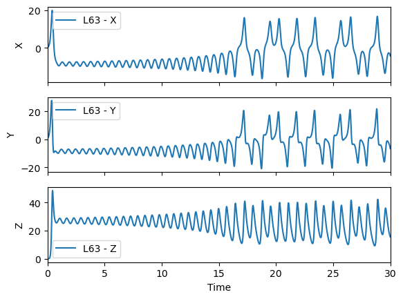
We first stick to Lorenz’s original choice of parameters and initial condition, and pick

\[\begin{split} \begin{eqnarray} \pr&=&10, \label{eq:lorpar1}\\ \lrayleigh&=&28, \label{eq:lorpar2}\\ b&=&8/3. \label{eq:lorpar3} \end{eqnarray} \end{split}\]

The equations are integrated numerically using a standard explicit integration scheme, known as the explicit Runge-Kutta scheme of order 4 (aka RK4), using the ode solver that comes with scipy (see the forwardModel.py python script) . This means in practice that the time axis is discretized, being divided into segments of width \(\tstep\); 4th order accuracy means that the error characterizing this numerical approximation is proportional to \(\tstep ^4\).

The piece of code below allows you to run the model and visualize the time evolution of \(X\), \(Y\) and \(Z\).

You can increase the value of the total integration time \(T\) to see the long-term evolution of the solution.

## Uncomment this line to make it interactive in JupyterLab!
# %matplotlib widget

import sys
import numpy as np
import forwardModel as fw
import matplotlib.pyplot as plt


# Getting familiar with Lorenz' 1963 model
# Control parameters 
rayleigh = 28 # Value of the Rayleigh number ratio 
prandtl = 10.
b = 8./3.

#integration time parameters
dt = 1.e-3      # This is the time step size
T = 30.         # Total integration time (in nondimensional time)
n_steps = int( np.ceil( T / dt)  )
time = np.linspace(0., T, n_steps + 1, endpoint=True) # array of discrete times

#initial condition
x0 = np.array( [0., 1., 0.], dtype=float )

#numerical integration given initial conditions and control parameters
x  = fw.forwardModel_r( x0, time, rayleigh, prandtl, b) 

#plot result
fig, ax = plt.subplots(nrows=3, ncols=1, sharex=True)
for k, comp in enumerate (["X","Y","Z"]):
    ax[k].plot(time, x[k,:], label='L63 - '+comp)
    ax[k].set_ylabel(comp)
    ax[k].legend()
ax[-1].set_xlabel('Time')
ax[-1].set_xlim(time[0],time[-1])
plt.show()

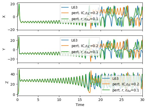
The Butterfly effect: sensitivity to a slight change in parameters or initial condition

Any change in the initial condition or control parameter will result in a solution that will diverge from the reference solution - this is the Butterfly effect, a hallmark of chaotic dynamical systems that makes long-term prediction of the dynamics of such systems impossible.

Below you can see how a change in the initial condition, by an amount \(\epsilon_{ic}\) affects the solution. In the code, the change affects the \(Y\) variable; feel free to apply it to the other variables, and also to vary its magnitude.

Likewise, let \(\epsilon_{par}\) be the amount by which the parameter \(\lrayleigh\) is changed. You can also visualize how this impacts the solution and play with its magnitude as well.

#Sensitivity to initial condition
#Change initial condition and compare solutions
epsilon_ic = 2.e-1 # feel free to change this value
x0 = np.array( [0., 1.+epsilon_ic, 0.], dtype=float )
x2  = fw.forwardModel_r( x0, time, rayleigh, prandtl, b) 

#Sensitivity to control parameters
epsilon_par = .1
x0 = np.array( [0., 1, 0.], dtype=float )
x3 = fw.forwardModel_r( x0, time, rayleigh+epsilon_par, prandtl, b) 

#Plot all three trajectories
fig, ax = plt.subplots(nrows=3, ncols=1, sharex=True)
for k, comp in enumerate (["X","Y","Z"]):
    ax[k].plot(time, x[k,:], label='L63')
    ax[k].plot(time, x2[k,:], label="pert. IC,$\epsilon_{IC}$="+str(epsilon_ic))
    ax[k].plot(time, x3[k,:], label="pert. $r$, $\epsilon_{Ra}$="+str(epsilon_par)) # effect of changing the value of one control parameter, Ra
    ax[k].set_ylabel( comp )
    ax[k].legend( loc='best')
ax[-1].set_xlabel('Time')
ax[-1].set_xlim(time[0],time[-1])
plt.show()

For later for those interested

Plot the time evolution of the difference between the original solution by Lorenz and the one obtained with a perturbed initial condition using a logarithmic scale on the \(y\)-axis. Describe this evolution.