Application of the ensemble Kalman filter (EnKF) to Lorenz’s 1963 model

\[ \newcommand{\myd}{\mathrm{d}} \newcommand{\statev}{\mathbf{X}} \newcommand{\lrayleigh}{{\mathrm{r}}} \newcommand{\rayleigh}{{\mathrm{Ra}}} \newcommand{\pr}{\mathrm{Pr}} \newcommand{\adj}{T} \newcommand{\tstep}{\Delta t} \]

The goal now is to get familiar with the working of a sequential assimilation scheme, running a so called twin experiment: A true, reference model trajectory \(\statev_i^t\) is generated (\(t\) stands for true, \(i\) for the discrete time index). The reference trajectory is used to construct a catalog of synthetic observations. These observations are then assimilated in order to correct a second model trajectory, which differs from the first one (the true one). In our case it will differ because we will assume a different initial condition, \(\statev_0 \neq \statev_0^t\).

Twin experiments (also called OSSE, Observing System Assimilation Experiments) are a logical first step when implementing an assimilation scheme, since they allow to develop an understanding for the behaviour of the scheme, without the additional complexity which may arise from the inability of the forward model to represent some of the physics expressed in the observations.

Today we will run these twin experiments using Lorenz’s 1963 model, and we will resort to the ensemble Kalman filter, which is a standard sequential assimilation scheme.

## Uncomment this line to make it interactive in JupyterLab!
#%matplotlib widget

import numpy as np
import forwardModel as fw
import matplotlib.pyplot as plt
from myEnKF import myEnKF

Definition of the reference trajectory

# We define the control parameters here 
rayleigh = 35 # 
prandtl = 10.
b = 8./3.

#initial condition for the true reference trajectory
x0 = np.array( [0., 1., 2.], dtype=float )

#integration time parameter
dt = 1.e-3      # This is time step size
T = 25.         # Total integration time, can be as short as 10 to speed things up
n_steps = int( np.ceil( T / dt)  )
time = np.linspace(0., T, n_steps + 1, endpoint=True) # array of discrete times

#numerical integration given initial conditions and control parameters
xt = fw.forwardModel_r( x0, time, rayleigh, prandtl, b) 

Creation of the catalog of synthetic observations

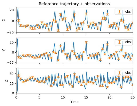
This is where we specify which variables are observed (we can decide that 1, 2 or even all 3 of them are measured), how often, and how accurate these observations are. To this end, we add an observation noise to the true value of the field of interest. This noise is assumed to be Gaussian, with standard deviation \(\sigma_{obs}\).

## How often do we observe the true state? 
dtobs = 0.5 # time between observations
# Which variables do we observe? 
WhichVariablesAreObserved = np.array( [1, 1, 1], dtype=float )
                    #  Determines which variables are available to
                    #  the EnKF. For example:
                    #  WhichVariablesAreObserved = [1 1 1]; 
                    #  means: X, Y, Z are observed
                    #  WhichVariablesAreObserved = [1 0 1];
                    #  means: X and Z are observed
                    #  WhichVariablesAreObserved = [1 0 0];
                    # means: X is observed
sigobs = 2.  # standard deviation of the observation noise
# We generate the synthetic data 
#  Construct observation matrix H
#  ........................................................................
H = np.diag( WhichVariablesAreObserved )

y_size = int( np.sum( WhichVariablesAreObserved ) )
H = np.zeros( (y_size, 3), dtype=float)
iy = 0
for ix in range(3):
    if WhichVariablesAreObserved[ix] > 0:
        H[iy,ix] = 1.
        iy = iy + 1

nobs = int( np.ceil( T / dtobs ) ) - 1  # number of times observations are performed
                                        # no observation at t=0 
gap  = int( dtobs/dt )# number of time steps between each observation 
time_obs = time[gap::gap]
# Generate vector of observations
y = np.zeros( (y_size, nobs), dtype=float)
R = np.diag( np.tile(sigobs**2, y_size) )
sqrt_s = np.sqrt(R)
# y = Hxt 
y = np.dot( H, xt[:,gap::gap] )
# compute observation error 
noise = np.dot(sqrt_s , np.random.normal( loc=0., scale=1.0, size=np.shape(y) ) )
# y = Hxt + epsilon 
y = y + noise

# Plot reference trajectory and the observations that will be fed to the EnKF 
fig, ax = plt.subplots(nrows=3, ncols=1, sharex=True)
iobs = 0
for k, comp in enumerate (["X","Y","Z"]):
    ax[k].plot(time, xt[k,:])
    if WhichVariablesAreObserved[k] > 0:
        ax[k].errorbar(time_obs, y[iobs,:], yerr=sqrt_s[iobs,iobs], fmt='o', markersize=3, capsize=4, label='obs')
        ax[k].legend(bbox_to_anchor=(1.01, 1),loc='upper right', frameon=True)
        iobs = iobs + 1
    ax[k].set_ylabel(comp)
ax[-1].set_xlabel('Time')
ax[-1].set_xlim(time[0],time[-1])
ax[0].set_title('Reference trajectory + observations')
plt.show()

Application of the Ensemble Kalman Filter

We will now assimilate these observations into a model whose trajectory will be hopefully drawn towards the true one, trough the sequential assimilation of data.

The ensemble, which is assumed to be centered on a zero initial condition, is characterized by

• its size (\(N_e\) is the number of elements of the ensemble),

• its initial spread that is also assumed to follow Gaussian statistics, with a standard deviation denoted by \(\sigma_{ens}\)

# Initialization of the Ensemble
Ne = 50                  # Number of ensemble members  
x0ens = np.array( [0.,0.,0.], dtype=float ) # The ensemble is centered on a zero initial condition
sigens = 10          # standard deviation of the ensemble
# initial covariance matrix
P0 =(sigens**2)*np.eye(3, dtype=float)

We have all the ingredients we need (physical model, observations, their statistics, initial ensemble) to apply the EnKF. The python script myEnKF.py contains the implementation of the EnKF. It returns two numpy arrays:

• xEnKF, which is the trajectory of the ensemble average - our guess of the trajectory

• x_ens, which contains the individual trajectories of the \(N_e\) ensemble members

#Now we run the EnKF 
xEnKF, x_ens = myEnKF( n_steps, dt, nobs, time_obs, gap, Ne, H, R, y, x0ens, P0, rayleigh, prandtl, b)

Since we are dealing with a twin experiment, we know what the true dynamical trajectory is, and we can assess exactly how good the EnKF is performing, under the conditions that were prescribed above.

The python code below is used to quantify the error, for the \(X\), \(Y\) and \(Z\) components of the state vector considered separately, and the 3 components taken together.

# Compute Euclidean error wrt true state which is known in this synthetic game
# cumulative error
cum_error_comp = np.sqrt( np.sum( (xt - xEnKF)**2, axis=1) ) 
cum_error      = np.sqrt( np.sum( cum_error_comp**2) )
norm_comp = np.sqrt( np.sum( xt**2, axis=1) ) 
norm      = np.sqrt( np.sum( norm_comp**2) )
print()
print(" Relative errors in %")
for k, comp in enumerate (["X","Y","Z"]):
    print("  "+(comp+"-component: %4.1f  ") % ( 100.*cum_error_comp[k]/norm_comp[k]) )
print()
print(("  3-component: %4.1f  ") % ( 100.*cum_error / norm  ) )

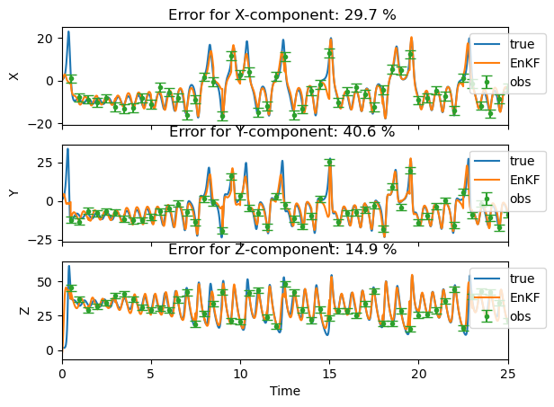
 Relative errors in %
  X-component: 34.5  
  Y-component: 42.1  
  Z-component: 14.5  

  3-component: 20.3  

We plot the results of the assimilation with the EnKF. For each component, the plots comprise the reference trajectory, the observations used for assimilation, and the EnKF estimate of the trajectory (the ensemble average). The legend also features the relative erros that were just computed.

By setting the plot_ensemble variable to True, you have the possibility to visualize individual trajectories as well (thin black lines).

#Plot results
plot_ensemble = False # Change to True if you want to visualize ensemble members
fig, ax = plt.subplots(nrows=3, ncols=1, sharex=True)
iobs = 0
for k, comp in enumerate (["X","Y","Z"]):
    ax[k].plot(time, xt[k,:], label='true')
    ax[k].plot(time, xEnKF[k,:], label='EnKF')
    if plot_ensemble is True:
        for e in range(Ne):
            ax[k].plot(time, x_ens[k,:,e], c='k', lw=0.1, zorder=-4)
    if WhichVariablesAreObserved[k] > 0:
        ax[k].errorbar(time_obs, y[iobs,:], yerr=sqrt_s[iobs,iobs], fmt='o', markersize=3, capsize=4, label='obs')
        iobs = iobs + 1
    ax[k].legend(bbox_to_anchor=(0.9, 1),loc='upper left', frameon=True)
    ax[k].set_ylabel(comp)
    ax[k].title.set_text( ("Error for "+comp+"-component: %4.1f %% ") % ( 100.*cum_error_comp[k]/norm_comp[k])  )
ax[-1].set_xlabel('Time')
ax[-1].set_xlim(time[0],time[-1])
plt.show()

Some questions

To address those questions, note that you must rerun the cells above as soon as you vary one parameter. Easiest way to do it is probably to use the ‘Restart kernel and run all cells’ in the Kernel tab.

Q1: All other parameters remaining constant, find the maximum value of \(\sigma_{obs}\) which leads to an acceptable behaviour of the EnKF (after you define what you consider an acceptable behaviour of the EnKF). One significant digit is enough.

Q2: Now with all other parameters remaining constant (σobs being equal to the value you just found),find the largest value of \(dt_{obs}\) (with 0.2 accuracy, say) which leads to an acceptable behaviour of the EnKF.

Q3: Is there a connection between this value and the typical time scale of the dynamics of the model?

Q4: Set \(dt_{obs}\) to half the maximum value you just found. Keeping all the other parameter constant, assume now that only X or Y is observed. Comment on the quality of the EnKF estimate based on either option.

Q5: It may be that the quality of the results depend strongly on the variable which is observed (X or Y). Would you have an explanation for this, based on a simple analysis of the equations that govern the dynamics of the L63 model?

Q6: All other parameters remaining constant, find the minimum number of elements of the ensemble \(N_e\) which leads to a good behaviour of the EnKF.

Q7: What conclusions do you draw from practising from the EnKF?