Swarm Measurements

Following on from the previous notebook, Making a main field model, in this demo we will access Swarm data and make a model in a similar way using data from space instead of ground observatories.

import datetime as dt
import numpy as np
import xarray as xr
import matplotlib.pyplot as plt
import cartopy.crs as ccrs
import cartopy.feature as cfeature
import holoviews as hv
import hvplot.xarray

from viresclient import SwarmRequest
from chaosmagpy.model_utils import design_gauss, synth_values

Fetching data to use

We fetch data as follows:

• MAGA_LR product from Swarm: this is the magnetic low rate (1Hz) data from Swarm Alpha

• the B_NEC variable is the field vector in the NEC (North, East, Centre) frame

• MLT: Magnetic Local Time of each measurement

• downsampled to one measurement per 10 seconds (PT10S)

• retaining only nominal measurements (according to Flags_B and Flags_F)

• during geomagnetically quiet times (Kp ≤ 2)

• during January 2020

request = SwarmRequest()
request.set_collection("SW_OPER_MAGA_LR_1B")
request.set_products(
    measurements=["B_NEC"],
    sampling_step="PT10S",
    auxiliaries=["MLT"],
)
request.set_range_filter("Flags_B", 0, 1)
request.set_range_filter("Flags_F", 0, 1)
request.set_range_filter("Kp", 0, 2)
data = request.get_between(
    start_time=dt.datetime(2020,1,1),
    end_time=dt.datetime(2020,2,1)
)
ds = data.as_xarray()
ds.attrs.pop("Sources")
ds

<xarray.Dataset>
Dimensions:     (Timestamp: 223946, NEC: 3)
Coordinates:
  * Timestamp   (Timestamp) datetime64[ns] 2020-01-01 ... 2020-01-31T23:59:50
  * NEC         (NEC) <U1 'N' 'E' 'C'
Data variables:
    Spacecraft  (Timestamp) object 'A' 'A' 'A' 'A' 'A' ... 'A' 'A' 'A' 'A' 'A'
    Latitude    (Timestamp) float64 76.7 77.33 77.96 ... -34.33 -34.97 -35.61
    Radius      (Timestamp) float64 6.803e+06 6.803e+06 ... 6.819e+06 6.819e+06
    B_NEC       (Timestamp, NEC) float64 3.137e+03 390.0 ... -2.472e+04
    MLT         (Timestamp) float64 6.569 6.595 6.623 ... 15.53 15.55 15.57
    Longitude   (Timestamp) float64 103.0 103.6 104.2 ... -128.1 -128.1 -128.1
Attributes:
    MagneticModels:  []
    AppliedFilters:  ['Flags_B <= 1', 'Flags_B >= 0', 'Flags_F <= 1', 'Flags_...

xarray.Dataset

• Dimensions:
  • Timestamp: 223946
  • NEC: 3
• Coordinates: (2)
  • Timestamp
    (Timestamp)
    datetime64[ns]
    2020-01-01 ... 2020-01-31T23:59:50

    description :

    Time stamp

    array(['2020-01-01T00:00:00.000000000', '2020-01-01T00:00:10.000000000',
           '2020-01-01T00:00:20.000000000', ..., '2020-01-31T23:59:30.000000000',
           '2020-01-31T23:59:40.000000000', '2020-01-31T23:59:50.000000000'],
          dtype='datetime64[ns]')

  • NEC
    (NEC)
    <U1
    'N' 'E' 'C'

    units :

    description :

    NEC frame - North, East, Centre (down)

    array(['N', 'E', 'C'], dtype='<U1')

• Data variables: (6)
  • Spacecraft
    (Timestamp)
    object
    'A' 'A' 'A' 'A' ... 'A' 'A' 'A' 'A'

    units :

    -

    description :

    Spacecraft identifier (values: 'A', 'B', 'C' or '-' if not available).

    array(['A', 'A', 'A', ..., 'A', 'A', 'A'], dtype=object)

  • Latitude
    (Timestamp)
    float64
    76.7 77.33 77.96 ... -34.97 -35.61

    units :

    deg

    description :

    Position in ITRF - Latitude

    array([ 76.6969509,  77.3277972,  77.95722  , ..., -34.326533 ,
           -34.9676442, -35.6087202])

  • Radius
    (Timestamp)
    float64
    6.803e+06 6.803e+06 ... 6.819e+06

    units :

    m

    description :

    Position in ITRF - Radius

    array([6802939.91, 6802905.25, 6802872.48, ..., 6818715.6 , 6818768.1 ,
           6818819.69])

  • B_NEC
    (Timestamp, NEC)
    float64
    3.137e+03 390.0 ... -2.472e+04

    units :

    nT

    description :

    Magnetic field vector, NEC frame

    array([[  3136.8997,    389.9523,  48679.9838],
           [  2950.7932,    419.6909,  48618.3234],
           [  2751.5652,    413.1472,  48556.8288],
           ...,
           [ 19715.5029,   6760.6679, -23862.4615],
           [ 19553.2631,   6832.909 , -24292.4989],
           [ 19389.2333,   6905.1276, -24718.6961]])

  • MLT
    (Timestamp)
    float64
    6.569 6.595 6.623 ... 15.55 15.57

    units :

    h

    description :

    Magnetic local time

    array([ 6.56885147,  6.59482384,  6.62251854, ..., 15.53264046,
           15.5511322 , 15.56994247])

  • Longitude
    (Timestamp)
    float64
    103.0 103.6 104.2 ... -128.1 -128.1

    units :

    deg

    description :

    Position in ITRF - Longitude

    array([ 103.042583 ,  103.5889765,  104.1958748, ..., -128.0893527,
           -128.087523 , -128.085006 ])

• Indexes: (2)
  • Timestamp
    PandasIndex

    PandasIndex(DatetimeIndex(['2020-01-01 00:00:00', '2020-01-01 00:00:10',
                   '2020-01-01 00:00:20', '2020-01-01 00:00:30',
                   '2020-01-01 00:00:40', '2020-01-01 00:00:50',
                   '2020-01-01 00:01:00', '2020-01-01 00:01:10',
                   '2020-01-01 00:01:20', '2020-01-01 00:01:30',
                   ...
                   '2020-01-31 23:58:20', '2020-01-31 23:58:30',
                   '2020-01-31 23:58:40', '2020-01-31 23:58:50',
                   '2020-01-31 23:59:00', '2020-01-31 23:59:10',
                   '2020-01-31 23:59:20', '2020-01-31 23:59:30',
                   '2020-01-31 23:59:40', '2020-01-31 23:59:50'],
                  dtype='datetime64[ns]', name='Timestamp', length=223946, freq=None))

  • NEC
    PandasIndex

    PandasIndex(Index(['N', 'E', 'C'], dtype='object', name='NEC'))

• Attributes: (2)

  MagneticModels :

  []

  AppliedFilters :

  ['Flags_B <= 1', 'Flags_B >= 0', 'Flags_F <= 1', 'Flags_F >= 0', 'Kp <= 2', 'Kp >= 0']

_ds = ds.drop("Timestamp").sel(NEC="C")
_ds.hvplot.scatter(
    x="Longitude", y="Latitude", color="B_NEC",
    rasterize=True, colorbar=True, cmap="coolwarm", clabel="Vertical (downwards) magnetic field (nT)"
)

Above, we show the vertical (downwards) component of the magnetic field vector sampled across Earth. If you zoom in, you can see the lines curving as the orbits converge over the poles. As we have taken a whole month of data, the spatial coverage is quite dense.

Building a model

Just as before, we perform a least-squares inversion to find Gauss coefficients.

In this case, we can easily go to higher spherical harmonic degree because we have many more data and they are globally distributed.

def build_model(ds, nmax=13):
    """Use the contents of dataset, ds, to build a SH model"""
    # Get the positions and measurements from ds
    radius = (ds["Radius"]/1e3).values
    theta = (90-ds["Latitude"]).values
    phi = (ds["Longitude"]).values
    B_radius = -ds["B_NEC"].sel(NEC="C").values
    B_theta = -ds["B_NEC"].sel(NEC="N").values
    B_phi = ds["B_NEC"].sel(NEC="E").values
    # Use ChaosMagPy to build the design matrix, G
    # https://chaosmagpy.readthedocs.io/en/master/functions/chaosmagpy.model_utils.design_gauss.html
    G_radius, G_theta, G_phi = design_gauss(radius, theta, phi, nmax=nmax)
    # Using only the radial component, perform the inversion:
    G = G_radius
    d = B_radius
    m = np.linalg.inv(G.T @ G) @ (G.T @ d)
    return m

model_coeffs = build_model(ds)

# The first 10 coefficients
model_coeffs[:10]

array([-29408.57813786,  -1450.96412916,   4652.73013794,  -2501.85494395,
         2981.30427171,  -2992.90080117,   1676.70095251,   -735.6252489 ,
         1363.59123489,  -2380.84233885])

Let’s sample our model and visualise it with contours:

def sample_model_on_grid(m, radius=6371.200):
    """Evaluate Gauss coefficients over a regular grid over Earth"""
    theta = np.arange(1, 180, 1)
    phi = np.arange(-180, 180, 1)
    theta, phi = np.meshgrid(theta, phi)
    B_r, B_t, B_p = synth_values(m, radius, theta, phi)
    ds_grid = xr.Dataset(
        data_vars={"B_NEC_model": (("y", "x", "NEC"), np.stack((-B_t, B_p, -B_r), axis=2))},
        coords={"Latitude": (("y", "x"), 90-theta), "Longitude": (("y", "x"), phi), "NEC": np.array(["N", "E", "C"])}
    )
    return ds_grid

# Evaluate at the mean radius of the satellite measurements
mean_radius_km = float(ds["Radius"].mean())/1e3
ds_grid = sample_model_on_grid(model_coeffs, radius=mean_radius_km)
# Generate contour plot of vertical component
ds_grid.sel(NEC="C").hvplot.contourf(
    x="Longitude", y="Latitude", c="B_NEC_model",
    levels=30, coastline=True, projection=ccrs.PlateCarree(), global_extent=True,
    clabel="Model: vertical (downwards) magnetic field (nT)"
)

/opt/conda/lib/python3.9/site-packages/geoviews/operation/projection.py:79: ShapelyDeprecationWarning: Iteration over multi-part geometries is deprecated and will be removed in Shapely 2.0. Use the `geoms` property to access the constituent parts of a multi-part geometry.
  polys = [g for g in geom if g.area > 1e-15]

Nice! It looks like the main field: a curved magnetic equator dropping southwards over South America (around the South Atlantic Anomaly where the field is weaker), the South magnetic pole occurs over the edge of Antarctica towards Australia, the North magnetic pole is more extended over Northern Canada and Siberia. Though it is not as accurate as published models!

Data-model residuals

Now let’s dig a little deeper, comparing the input data and the model…

Let’s plot the difference between the data and the model, the “data-model residuals”:

# Evaluate the model at the same points as the measurements
def append_model_evaluations(ds, m):
    ds = ds.copy()
    B_r, B_t, B_p = synth_values(m, ds["Radius"]/1e3, 90-ds["Latitude"], ds["Longitude"])
    ds["B_NEC_model"] = ("Timestamp", "NEC"), np.stack((-B_t, B_p, -B_r), axis=1)
    ds["B_NEC_res_model"] = ds["B_NEC"] - ds["B_NEC_model"]
    return ds
ds = append_model_evaluations(ds, model_coeffs)

# Plot the 
_ds = ds.drop("Timestamp").sel(NEC="C")
_ds.hvplot.scatter(
    x="Longitude", y="Latitude", color="B_NEC_res_model",
    rasterize=True, colorbar=True, cmap="coolwarm", clim=(-40, 40), clabel="Vertical (B_C) data-model residuals (nT)",
)

(Above): The difference between the model and the data is quite small except over the poles… let’s look at the other components now:

_ds = ds.drop("Timestamp").sel(NEC="E")
_ds.hvplot.scatter(
    x="Longitude", y="Latitude", color="B_NEC_res_model",
    rasterize=True, colorbar=True, cmap="coolwarm", clim=(-40, 40), clabel="Eastward (B_E) data-model residuals (nT)",
)

(Above): The disturbance over the poles is much stronger in the Eastward component… this is related to the geometry of the field-aligned currents producing a larger magnetic perturbation in that direction.

Next let’s plot against magnetic local time (MLT) instead, as the relevant coordinate system in which these currents are organised:

_ds = ds.drop("Timestamp").sel(NEC="E")
_ds.hvplot.scatter(
    x="MLT", y="Latitude", color="B_NEC_res_model",
    rasterize=True, colorbar=True, cmap="coolwarm", clim=(-40, 40), clabel="Eastward (B_E) data-model residuals (nT)",
)

ds.drop("Timestamp").hvplot.scatter(x="Latitude", y="B_NEC_res_model", col="NEC", rasterize=True, colorbar=False, cmap="bwr")

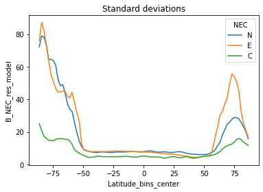
(Above): Both the Northward (N) and Eastward (E) components are more disturbed over the poles than the downward (C) component. This disturbance is due to Field-Aligned Currents (FACs) and Auroral Electrojets (AEJs) which produce strong magnetic fields over the poles.

fig, ax = plt.subplots(1, 1)
(ds.groupby_bins("Latitude", 90)
   .apply(lambda x: x["B_NEC_res_model"].std(axis=0))
   .plot.line(x="Latitude_bins", ax=ax)
)
ax.set_title("Standard deviations");

Exercises

• Plot the power spectrum of our model

• See what happens if you try push it to higher SH degree

• Alter the inversion to use other components (the one here only used the vertical component)

Exploring further

Take a look at Swarm Notebooks if you want more examples. There you will also find recipes for accessing other Swarm products.