Making a main field model

Making a main field model#

Here we demonstrate how to make a simple time-independent main field model by fitting spherical harmonics to ground observatory measurements.

The principles of spherical harmonic analysis have been shown in the previous pages, so here we will take a shortcut and use utilties from ChaosMagPy

Clemens Kloss et al. (2025). ancklo/ChaosMagPy: ChaosMagPy v0.15 (v0.15). Zenodo. https://doi.org/10.5281/zenodo.16091680

We will use:

design_gauss to generate the design matrix for the inversion
synth_values to run the forward model to get predictions for the magnetic field from our model

hvPlot is used to create some fancy visualisations but this library is more complex to use! so if you are newer to the Python ecosystem, you are better off using Matplotlib for your own work.

# Install pooch (not currently in VRE)
%pip install pooch

import pooch
from chaosmagpy.model_utils import design_gauss, synth_values, power_spectrum
from chaosmagpy.plot_utils import plot_power_spectrum
import numpy as np
import pandas as pd
import xarray as xr
import matplotlib.pyplot as plt
import cartopy.crs as ccrs
import cartopy.feature as cfeature
import hvplot.xarray

ERROR 1: PROJ: proj_create_from_database: Open of /opt/conda/share/proj failed

Building a model#

Suppose we have data, $\vec{d}$ (i.e. the set of magnetic measurements), and we want to find a model $\vec{m}$ (i.e. a set of Gauss coefficients, $[\begin{matrix} g_{n}^{m} & h_{n}^{m} \end{matrix}]$ , to be determined), we can connect these with a matrix $G$ (the so-called design matrix):

\vec{d} = G \vec{m}

$G$ can be constructed by comparing to the spherical harmonic expansion of the magnetic field $\vec{B}$ (where we have neglected external sources for simplicity):

\begin{array}{r} \begin{aligned} \vec{d} = & G \vec{m} \\ B_{i} = & G [\begin{array}{c} g_{n}^{m} & h_{n}^{m} \end{array}] \\ B_{i} = & - \partial_{i} (R_{E} \sum_{n = 1}^{N} \sum_{m = 0}^{n} (g_{n}^{m} \cos m ϕ + h_{n}^{m} \sin m ϕ) {(\frac{R_{E}}{r})}^{n + 1} P_{n}^{m} (\cos θ)) \\ = & - \partial_{i} [\begin{array}{c} R_{E} \sum_{n = 1}^{N} \sum_{m = 0}^{n} (\cos m ϕ) {(\frac{R_{E}}{r})}^{n + 1} P_{n}^{m} (\cos θ) \\ R_{E} \sum_{n = 1}^{N} \sum_{m = 0}^{n} (\sin m ϕ) {(\frac{R_{E}}{r})}^{n + 1} P_{n}^{m} (\cos θ) \end{array}] [\begin{array}{c} g_{n}^{m} & h_{n}^{m} \end{array}] \end{aligned} \end{array}

Note that:

$B_{i}$ are the three vector components, $(B_{r}, B_{θ}, B_{ϕ}) = (- B_{C}, - B_{N}, B_{E})$ , i.e. the data, $\vec{d}$
$\partial_{i}$ is a shorthand which should be replaced by the derivatives in spherical polar coordinates $(\partial_{r} = \frac{\partial}{\partial r}, \partial_{θ} = \frac{1}{r} \frac{\partial}{\partial θ}, \partial_{ϕ} = \frac{1}{r \sin θ} \frac{\partial}{\partial ϕ})$
$[\begin{matrix} g_{n}^{m} & h_{n}^{m} \end{matrix}]$ are the Gauss coefficients, i.e. the model, $\vec{m}$

A least-squares solution to $\vec{d} = G \vec{m}$ can be found with:

\vec{m} = (G^{T} G)^{- 1} G^{T} \vec{d}

# Identify coordinates and measurements
theta = input_data["Colat"]
phi = input_data["Long"]
radius = 6371.2 + input_data["alt(m)"]/1e3
B_radius = -input_data["Z"]
B_theta = -input_data["X"]
B_phi = input_data["Y"]

# Build the design matrix
N_max = 6
G_radius, G_theta, G_phi = design_gauss(radius, theta, phi, nmax=N_max, source="internal")

# Perform the inversion
G = np.concatenate((G_radius, G_theta, G_phi))
d = np.concatenate((B_radius, B_theta, B_phi))
m = np.linalg.inv(G.T @ G) @ (G.T @ d)
m

array([-2.98706210e+04, -1.72878664e+03,  5.10437604e+03, -2.36677354e+03,
        3.21808504e+03, -2.60186018e+03,  1.81146058e+03, -4.40900880e+02,
        1.20096209e+03, -2.28721723e+03, -2.58558551e+02,  1.28174523e+03,
        2.26792327e+02,  7.08225964e+02, -5.55967072e+02,  8.56002210e+02,
        8.54262291e+02,  1.88225598e+02,  2.21210848e+02, -1.75262151e+02,
       -3.56256647e+02,  2.20607631e+02,  1.12133919e+02, -3.04804983e+02,
       -2.21046651e+02,  1.77423732e+02, -2.70829977e+01,  2.26917637e+02,
        1.30066476e+02, -1.93969550e+01, -1.25596377e+02, -1.97358431e+02,
        5.34487565e+00,  5.21247100e+01,  1.36761971e+02,  8.68218607e+01,
       -1.15948032e+01, -1.82150875e+02,  3.19243839e+02, -5.68244622e+01,
       -7.25136804e+01,  1.65716700e+02, -6.60842751e+01, -5.59273212e+01,
       -9.38254025e+00,  2.39803027e+01, -1.40908041e+02,  1.34255677e+01])

Since we do not have many data, we would need to be more sophisticated with the inversion procedure (e.g. including regularisation) to get a model of higher resolution. For this reason, the model is truncated at spherical harmonic degree 6. You can explore increasing this limit.

Exercise#

What is the shape of the design matrix?
What is the amplitude of the axial dipole ( $g_{0}^{1}$ ) and how does it compare with the IGRF?

How good is our model?#

Let’s evaluate the model over the Earth and plot contours…

def build_model(ds=input_data, nmax=10):
    """Returns Gauss coefficients for a simple SH model"""
    theta = ds["Colat"]
    phi = ds["Long"]
    radius = 6371.2 + ds["alt(m)"]/1e3
    B_radius = -ds["Z"]
    B_theta = -ds["X"]
    B_phi = ds["Y"]
    # Build the design matrix
    G_radius, G_theta, G_phi = design_gauss(radius, theta, phi, nmax=nmax, source="internal")
    # Perform the inversion
    G = np.concatenate((G_radius, G_theta, G_phi))
    d = np.concatenate((B_radius, B_theta, B_phi))
    m = np.linalg.inv(G.T @ G) @ (G.T @ d)
    return m


def sample_model_on_grid(m, radius=6371.200):
    """Evaluate Gauss coefficients over a regular grid over Earth"""
    theta = np.arange(1, 180, 1)
    phi = np.arange(-180, 180, 1)
    theta, phi = np.meshgrid(theta, phi)
    B_r, B_t, B_p = synth_values(m, radius, theta, phi)
    ds_grid = xr.Dataset(
        data_vars={"B_NEC_model": (("y", "x", "NEC"), np.stack((-B_t, B_p, -B_r), axis=2))},
        coords={"Latitude": (("y", "x"), 90-theta), "Longitude": (("y", "x"), phi), "NEC": np.array(["N", "E", "C"])}
    )
    return ds_grid


def plot_model_contours(m):
    ds_grid = sample_model_on_grid(m)
    # Generate contour plot of vertical component
    return ds_grid.sel(NEC="C").hvplot.contourf(
        x="Longitude", y="Latitude", c="B_NEC_model",
        levels=30, coastline=True, projection=ccrs.PlateCarree(), global_extent=True,
        clabel="Model: vertical (downwards) magnetic field (nT)"
    )


m = build_model(input_data, nmax=6)
plot_model_contours(m)

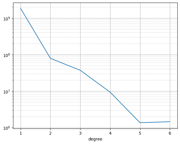
The power spectrum is a common way to assess and compare models, showing how much power is concentrated at each spherical harmonic degree. We can use plot_power_spectrum from ChaosMagPy:

plot_power_spectrum(power_spectrum(m));

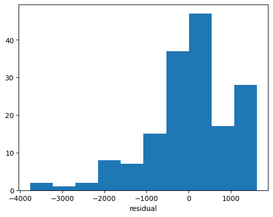
../_images/fab80e1a1f11e1d7259bee4c2d822d8c69c093bde14a8e2277d595a5831520dc.png

… and we can look at the residuals between the input data and the model:

def append_residuals(ds=input_data, m=m):
    # Evaluate model at the data locations
    B_r, B_t, B_p = synth_values(m, 6371.2 + ds["alt(m)"]/1e3, ds["Colat"], ds["Longitude"])
    # Assign data-model residuals to the dataset
    ds["res_N"] = ds["X"] - (-B_t)
    ds["res_E"] = ds["Y"] - (B_p)
    ds["res_C"] = ds["Z"] - (-B_r)
    return ds

ds = append_residuals(input_data, m)

plt.hist(ds["res_C"])
plt.xlabel("residual");

../_images/2dc48bbfe91a4cbe660e0a413398371eebd9fd0dd4021bf20bbb1489a0d2da07.png

ds.hvplot.scatter(
    x="Longitude", y="Latitude", c="res_C",
    coastline=True, projection=ccrs.PlateCarree(), global_extent=True,
    clabel="Data-model residual: vertical (downwards) magnetic field (nT)"
)

WARNING:param.main: geo option cannot be used with kind='scatter' plot type. Geographic plots are only supported for following plot types: ['bivariate', 'contour', 'contourf', 'dataset', 'hexbin', 'image', 'labels', 'paths', 'points', 'points', 'polygons', 'quadmesh', 'rgb', 'vectorfield']

/opt/conda/lib/python3.11/site-packages/xarray/core/utils.py:494: FutureWarning: The return type of `Dataset.dims` will be changed to return a set of dimension names in future, in order to be more consistent with `DataArray.dims`. To access a mapping from dimension names to lengths, please use `Dataset.sizes`.
  warnings.warn(

Exercise#

Calculate the RMS misfit for each vector component (Hint: we have stored the residuals in the dataset, accessible as ds["res_N"], ds["res_E"], ds["res_C"])
Experiment with changing the SH degree trunction in the model
Experiment with using data just over Europe
Add random noise into the data to observe the effect
Use viresclient to access the monthly means dataset and produce a model using those instead

def select_europe(ds=input_data):
    """Subselect the dataset down to just cover Europe"""
    colat_minmax = (20, 60)
    lon_minmax = (-10, 40)
    ds = ds.where(
        (ds["Colat"] > colat_minmax[0]) & (ds["Colat"] < colat_minmax[1]) &
        (ds["Long"] > lon_minmax[0]) & (ds["Long"] < lon_minmax[1]),
    ).dropna(dim="index")
    return ds

Making a main field model

Contents

Making a main field model#

Loading some data#

Building a model#

Exercise#

How good is our model?#

Exercise#