Satellite data selection#
import datetime as dt
import numpy as np
import xarray as xr
import matplotlib as mpl
import matplotlib.pyplot as plt
from mpl_toolkits.axes_grid1.inset_locator import inset_axes
import cartopy.crs as ccrs
import cartopy.feature as cfeature

from viresclient import SwarmRequest
ERROR 1: PROJ: proj_create_from_database: Open of /opt/conda/share/proj failed
Fetching Swarm data using VirES#
Magnetic field measurements from Swarm Alpha are available within the SW_OPER_MAGA_LR_1B dataset. Here we use the viresclient Python package to fetch these measurements.
def fetch_data():
    """Fetch Swarm data using the VirES service"""

    request = SwarmRequest()
    # Specify dataset to use
    request.set_collection("SW_OPER_MAGA_LR_1B")
    request.set_products(
        measurements=["B_NEC"],
        sampling_step="PT1M",  # Sample at 1-minute resolution
    )
    # Fetch 1 month of data
    data = request.get_between(
        start_time=dt.datetime(2025,1,1),
        end_time=dt.datetime(2025,2,1)
    )
    # Load data using xarray
    ds = data.as_xarray()
    ds.attrs.pop("Sources")
    return ds

ds_1 = fetch_data()
ds_1
<xarray.Dataset>
Dimensions:     (Timestamp: 44640, NEC: 3)
Coordinates:
  * Timestamp   (Timestamp) datetime64[ns] 2025-01-01 ... 2025-01-31T23:59:00
  * NEC         (NEC) <U1 'N' 'E' 'C'
Data variables:
    Spacecraft  (Timestamp) object 'A' 'A' 'A' 'A' 'A' ... 'A' 'A' 'A' 'A' 'A'
    Longitude   (Timestamp) float64 151.1 151.1 151.0 ... -68.91 -68.92 -68.9
    Radius      (Timestamp) float64 6.831e+06 6.83e+06 ... 6.835e+06 6.835e+06
    B_NEC       (Timestamp, NEC) float64 2.863e+04 1.556e+03 ... -1.321e+04
    Latitude    (Timestamp) float64 9.757 13.6 17.44 ... -29.19 -33.03 -36.86
Attributes:
    MagneticModels:  []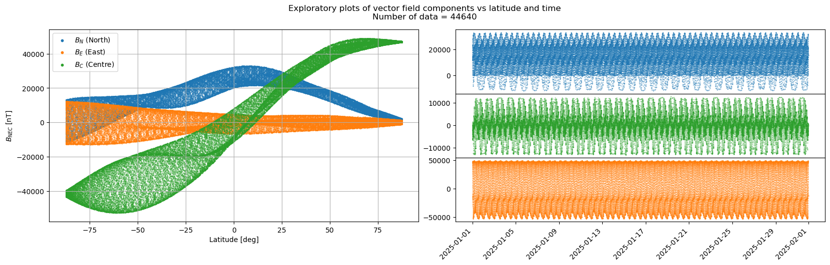
AppliedFilters: []Inspecting data#
def plot_data_preview(ds):
    """Plot magnetic field vector against latitude and time"""

    # Configure figure layout
    fig = plt.figure(figsize=(20, 5))
    gs = fig.add_gridspec(3, 2)
    ax_L0 = fig.add_subplot(gs[:, 0])
    ax_R0 = fig.add_subplot(gs[0, 1])
    ax_R1 = fig.add_subplot(gs[1, 1])
    ax_R2 = fig.add_subplot(gs[2, 1])
    # Left: Plot B_NEC vector components against latitude, on one figure
    ax_L0.scatter(x=ds["Latitude"], y=ds["B_NEC"].sel(NEC="N"), s=.1, label="$B_N$ (North)")
    ax_L0.scatter(x=ds["Latitude"], y=ds["B_NEC"].sel(NEC="E"), s=.1, label="$B_E$ (East)")
    ax_L0.scatter(x=ds["Latitude"], y=ds["B_NEC"].sel(NEC="C"), s=.1, label="$B_C$ (Centre)")
    ax_L0.set_ylabel("$B_{NEC}$ [nT]")
    ax_L0.set_xlabel("Latitude [deg]")
    ax_L0.grid()
    ax_L0.legend(markerscale=10)
    # Right: Plot B_NEC against time, over three figures
    ax_R0.scatter(x=ds["Timestamp"], y=ds["B_NEC"].sel(NEC="N"), s=.1, c="tab:blue")
    ax_R1.scatter(x=ds["Timestamp"], y=ds["B_NEC"].sel(NEC="E"), s=.1, c="tab:green")
    ax_R2.scatter(x=ds["Timestamp"], y=ds["B_NEC"].sel(NEC="C"), s=.1, c="tab:orange")
    # Adjust axes etc
    fig.subplots_adjust(wspace=.1, hspace=0)
    ax_R0.set_xticklabels([])
    ax_R1.set_xticklabels([])
    plt.setp(ax_R2.get_xticklabels(), rotation=45, ha='right')
    N_samples = len(ds["B_NEC"])
    fig.suptitle(f"Exploratory plots of vector field components vs latitude and time\nNumber of data = {N_samples}");

    return fig

fig_1 = plot_data_preview(ds_1)
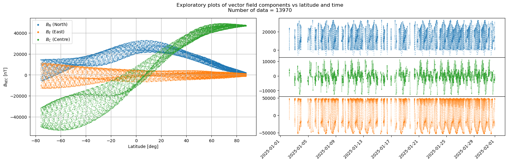
Selecting data to use for modelling#
Here we apply three types of data selection:
Data quality: Instrumental problems can occur and should(!) be indicated by the quality flags (
Flags_B,Flags_F,Flags_q)Geomagnetic activity: Select quiet periods based on Kp and rate of change of Dst
Sunlight: The dayside ionosphere is more active so we choose to use only nightside data
def fetch_selected_data():
    """Fetch Swarm data, using filters to select the "clean" measurements"""

    request = SwarmRequest()
    request.set_collection("SW_OPER_MAGA_LR_1B")
    request.set_products(
        measurements=["B_NEC"],
        sampling_step="PT1M",
        # auxiliaries=["Kp", "dDst", "MLT", "SunZenithAngle"],
    )
    # Reject bad data according to quality flags
    request.add_filter("Flags_B != 255")
    request.add_filter("Flags_q != 255")
    # Reject geomagnetically active times
    request.add_filter("Kp <= 3")
    request.add_filter("dDst <= 3")
    # Reject sunlit data (retain data where Sun is 10° below horizon)
    request.add_filter("SunZenithAngle >= 80")
    data = request.get_between(
        start_time=dt.datetime(2025,1,1),
        end_time=dt.datetime(2025,2,1)
        # start_time=dt.datetime(2018, 9, 14),
        # end_time=dt.datetime(2018, 9, 28)
    )
    ds = data.as_xarray()
    ds.attrs.pop("Sources")
    return ds

ds_2 = fetch_selected_data()
ds_2
<xarray.Dataset>
Dimensions:     (Timestamp: 13970, NEC: 3)
Coordinates:
  * Timestamp   (Timestamp) datetime64[ns] 2025-01-02T05:52:00 ... 2025-01-31...
  * NEC         (NEC) <U1 'N' 'E' 'C'
Data variables:
    Spacecraft  (Timestamp) object 'A' 'A' 'A' 'A' 'A' ... 'A' 'A' 'A' 'A' 'A'
    Longitude   (Timestamp) float64 64.87 65.24 65.76 ... -98.12 -82.3 -76.28
    Radius      (Timestamp) float64 6.823e+06 6.822e+06 ... 6.819e+06 6.819e+06
    B_NEC       (Timestamp, NEC) float64 1.299e+04 2.586e+03 ... 4.65e+04
    Latitude    (Timestamp) float64 55.45 59.29 63.12 ... 85.39 81.93 78.22
Attributes:
    MagneticModels:  []
AppliedFilters: ['Flags_B != 255', 'Flags_q != 255', 'Kp <= 3', 'SunZeni...fig_2 = plot_data_preview(ds_2)
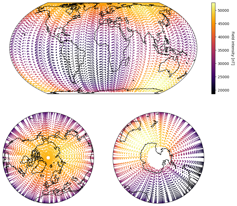
def global_plot(ds):
    """Plot intensity over the glob"""

    # Append intensity, F, to the dataset
    ds["F"] = np.sqrt((ds["B_NEC"]**2).sum(axis=1))

    fig = plt.figure(figsize=(10, 10))
    gs = fig.add_gridspec(2, 2)
    ax_N = fig.add_subplot(gs[1, 0], projection=ccrs.Orthographic(0,90))
    ax_S = fig.add_subplot(gs[1, 1], projection=ccrs.Orthographic(180,-90))
    ax_G = fig.add_subplot(gs[0, :], projection=ccrs.EqualEarth())

    for ax in (ax_N, ax_S, ax_G):
        pc = ax.scatter(
            ds["Longitude"], y=ds["Latitude"], c=ds["F"],
            s=5, edgecolors="none", cmap="inferno", transform = ccrs.PlateCarree()
        )
        ax.coastlines(linewidth=1.1)
    # Add colorbar inset axes into global map and move upwards
    cax = inset_axes(ax_G, width="2%", height="100%", loc="right", borderpad=-5)
    clb = plt.colorbar(pc, cax=cax)
    clb.set_label("Field intensity [nT]", rotation=270, va="bottom")

fig_3 = global_plot(ds_2)
Exercises#
Experiment with changing the selection criteria for Kp, dDst, solar zenith angle (hint: alter the line
request.add_filter("Kp <= 3"))Experiment using different months of data
How might the selection criteria bias the measurements?
Change the time period to:
start_time=dt.datetime(2018, 9, 14),
end_time=dt.datetime(2018, 9, 28)
(which we will use in the following notebook)