Tracing magnetic field lines#
# Import notebook dependencies
import os
import sys
import numpy as np
import pandas as pd
import matplotlib.pyplot as plt
%matplotlib inline

from src import sha, IGRF13_FILE
Tracing magnetic field lines#
The basic principle in following a field line at a point is to calculate the field vector there, then ‘take a step’ in the direction of the field to a new point, and repeat. The smaller the step, the higher the accuracy. This can be expressed as
with
Axisymmetric multipole field lines#
In this case there is no variation with longitude (
using spherical coordinates, which gives the equation of the field line as
This equation can be solved when the field is expressed in terms of spherical harmonics for the axisymmetric terms with
Note the power of spherical harmonic degree
For the field line that passes through a given starting position (
which gives the following expression for the scaling factor,
is derived.
The (un-normalised) forms of
These, along with the expression for
def dipole(r0, theta_0, th):      # P(n=1, m=0)
    k = r0/(np.sin(theta_0)**2)
    return (k*np.sin(th)**2)

def quadpole(r0, theta_0, th):    # P(n=2, m=0)
    k = r0**2/(np.sin(theta_0)**2*np.cos(theta_0))
    P = np.cos(th)*np.sin(th)**2
    return (np.sqrt(np.abs(k)*np.abs(P)))

def octpole(r0, theta_0, th):     # P(n=3, m=0)
    k = r0**3/(np.sin(theta_0)**2*(5*np.cos(theta_0)**2-1))
    P = (5*np.cos(th)**2-1)*np.sin(th)**2
    return ((np.abs(k)*np.abs(P))**(1/3))

def hexdpole(r0, theta_0, th):    # P(n=4, m=0)
    k = r0**4/((7*np.cos(theta_0)**3-3*np.cos(theta_0))*np.sin(theta_0)**2)
    P =(7*np.cos(th)**3-3*np.cos(th))*np.sin(th)**2
    return ((np.abs(k)*np.abs(P))**(1/4))
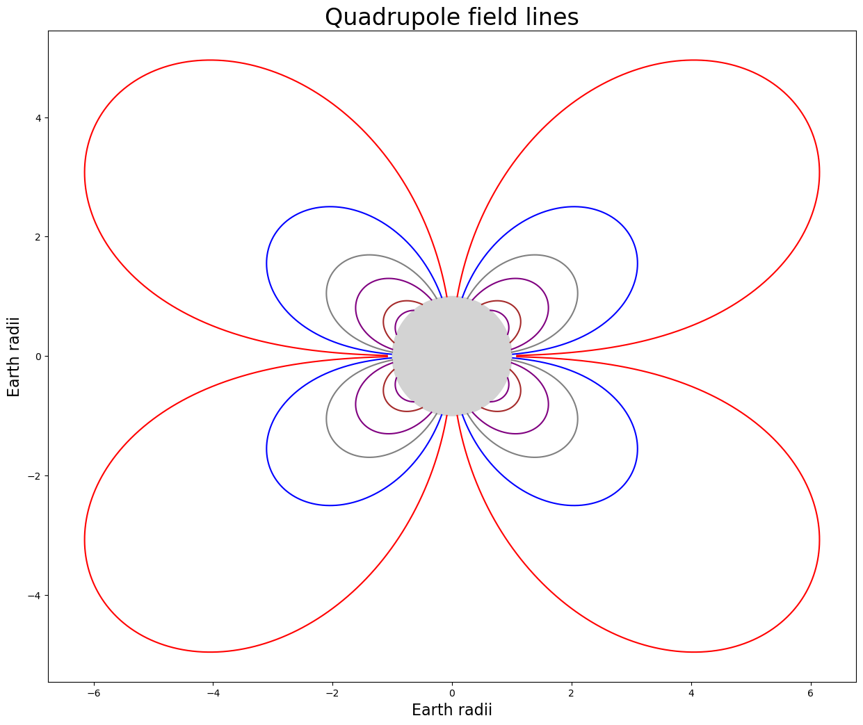
You can plot dipole, quadrupole, octupole and hexadecapole field lines using the code below. Start by choosing the type of multipole field lines to plot by setting the value of pole_type to the desired spherical harmonic degree
>> USER INPUT HERE: Set the plotting parameters below (pole type and starting colatitudes)#
pole_type options:
1 = dipole
2 = quadrupole
3 = octupole
4 = hexadecapole
# Pole type
pole_type = 2

# Experiment by changing a list of starting colatitudes
theta   = [5, 10, 15, 20, 30, 40]
Now create the plot.
d2r     = np.deg2rad
axpoles = {1:dipole, 2:quadpole, 3:octpole, 4:hexdpole}
names   = {1:'Dipole', 2:'Quadrupole', 3:'Octupole', 4:'Hexadecapole'}
clines  = ['red', 'blue', 'grey', 'purple', 'brown', 'purple', 'pink', 'orange', 'magenta', 'olive', 'cyan']

# Define the "Earth"
r0  = 1
the = d2r(np.linspace(0, 360, 1000))
xe  = r0*np.sin(the)
ye  = r0*np.cos(the)

fig, ax = plt.subplots(figsize=(15, 15))
ax.set_aspect('equal')
ax.fill(xe, ye, color='lightgrey') # Plot the Earth

ic = -1
for i in theta:
    ic += 1
    theta_0 = d2r(i)
    th = np.linspace(theta_0, d2r(90), 1000)
    rad = axpoles[pole_type](r0, theta_0, th)
    xb = rad*np.sin(th)
    yb = rad*np.cos(th)
    xb[np.where(rad<1)] = np.nan
    yb[np.where(rad<1)] = np.nan
    ax.plot(xb, yb, color = clines[ic%10])
    # Assume a symmetrical distribution in the four quadrants
    ax.plot( xb, -yb, color = clines[ic%10])
    ax.plot(-xb,  yb, color = clines[ic%10])
    ax.plot(-xb, -yb, color = clines[ic%10])
ax.set_xlabel('Earth radii', fontsize=16)
ax.set_ylabel('Earth radii', fontsize=16)
ax.set_title(names[pole_type]+' field lines', fontsize=24);
References#
Jeffreys, B. (1988) ‘Derivations of the equation for the field lines of an axisymmetric multipole’, Geophysical Journal International. John Wiley & Sons, Ltd (10.1111), 92(2), pp. 355–356. doi: 10.1111/j.1365-246X.1988.tb01148.x.
Willis, D. M. and Young, L. R. (1987) ‘Equation for the field lines of an axisymmetric magnetic multipole’, Geophysical Journal International. Oxford University Press, 89(3), pp. 1011–1022. doi: 10.1111/j.1365-246X.1987.tb05206.x.
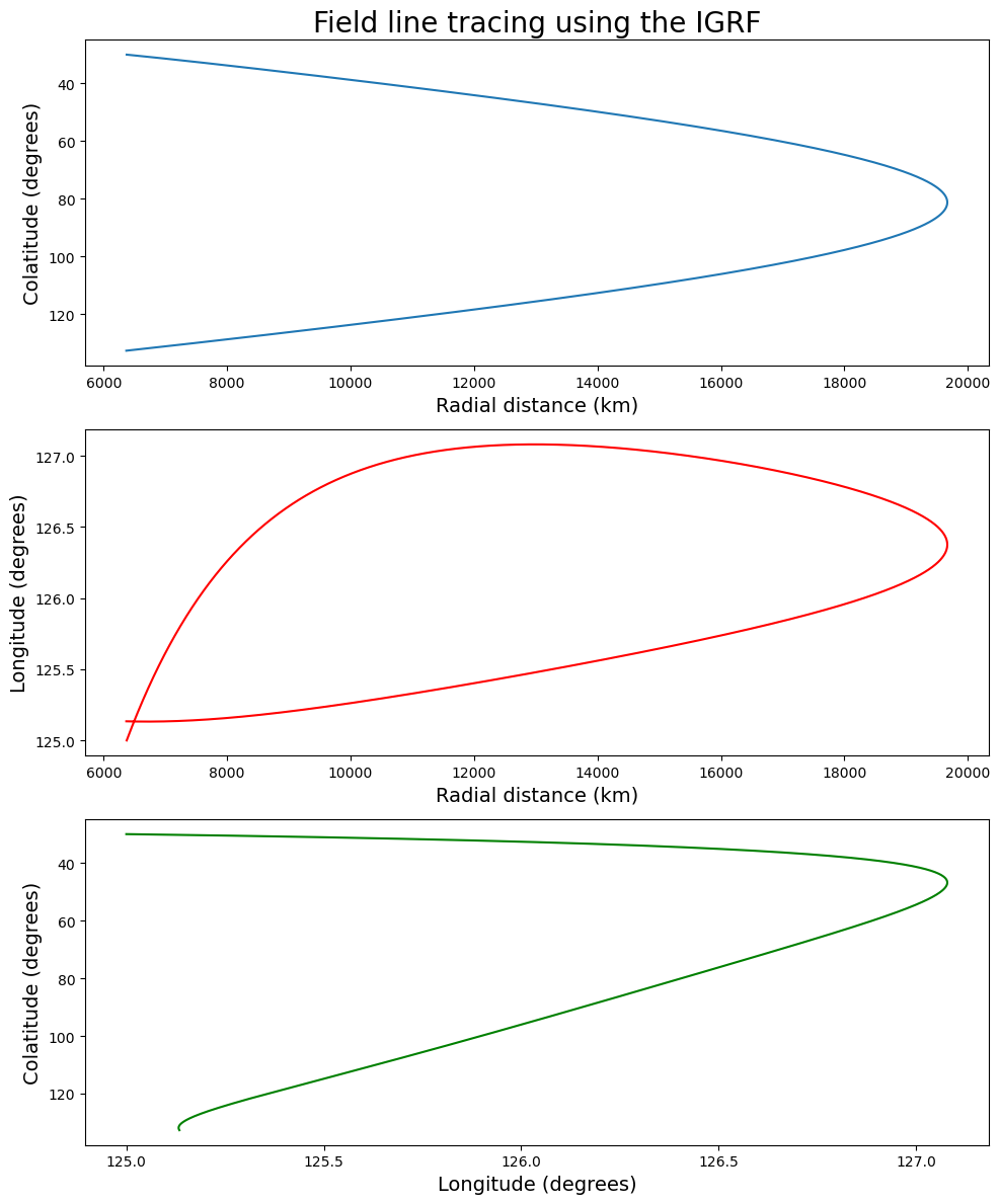
Using the IGRF to trace field lines (and find conjugate points)#
The IGRF gives a fuller 3-D representation of the geomagnetic field, rather than the axisymmetric 2-D representation used above, and so the ‘stepping strategy’ is needed to follow field lines. The dipole field dominates, as we would expect, but it is interesting to to see how the colatitude and longitude change along the path. The starting and ending points at the Earth’s surface are ‘connected’ by a field line - they are conjugate points. (The IGRF for 2020.0 is used in the code below.)
>> >> USER INPUT HERE: Set the input parameters (listed below)#
Starting colatitude (degrees)
Starting longitude (degrees)
Step size (km)
# Starting colatitude and longitude (east) in degrees
theta_0   = 30
phi_0     = 125

# Step size for the field line tracing in km
step_size = 10
Now do the calculation and plot the results. *** This may take a few seconds - be patient! ***
d2r = np.deg2rad
r2d = np.rad2deg
fcalc = lambda x: np.sqrt(np.dot(x,x))

igrf13 = pd.read_csv(IGRF13_FILE, delim_whitespace=True, header=3)
gh2020 = np.append(0., igrf13['2020.0'])
NMAX   = 13

# Initialise variables at starting point
r0      = 6371.2
thrd    = d2r(theta_0)
phrd    = d2r(phi_0)
track   = [(r0, thrd, phrd)]  # Store coordinates of points on the field line
bxyz    = sha.shm_calculator(gh2020, NMAX, r0, theta_0, phi_0, 'Geocentric')
eff     = fcalc(bxyz)
lamb    = step_size/eff
rad     = r0

# Allow a maximum number of steps in the iteration for the field line to
# return to the Earth's surface
maxstep = 10000
newrad  = r0+0.001

step    = 0
while step <= maxstep and newrad >= r0:
    rad, th, ph  =  track[step]
    lx,  ly, lz  =  tuple(el*lamb for el in bxyz)
    newrad = rad+lz
    newth  = th+lx/rad
    newph  = ph-ly/(rad*np.sin(th))
    track += [(newrad, newth, newph)]
    bxyz   =  sha.shm_calculator(gh2020, NMAX, newrad, r2d(newth), \
                                 r2d(newph),'Geocentric')
    lamb   =  step_size/fcalc(bxyz)
    step  += 1

rads = np.array([r[0] for r in track])
ths  = np.array([t[1] for t in track])
phs  = np.array([p[2] for p in track])

fig, (ax0, ax1, ax2) = plt.subplots(nrows=3, ncols=1, figsize=(10, 12))
ax0.plot(rads, r2d(ths))
ax0.invert_yaxis()
ax0.set_xlabel('Radial distance (km)', fontsize=14)
ax0.set_ylabel('Colatitude (degrees)', fontsize=14)
ax0.set_title('Field line tracing using the IGRF', fontsize=20)
ax1.plot(rads, r2d(phs), color='red')
ax1.set_xlabel('Radial distance (km)', fontsize=14)
ax1.set_ylabel('Longitude (degrees)', fontsize=14)
ax2.plot(r2d(phs), r2d(ths), color='green')
ax2.set_xlabel('Longitude (degrees)', fontsize=14)
ax2.set_ylabel('Colatitude (degrees)', fontsize=14)
ax2.invert_yaxis()
fig.tight_layout()
print('\nCoordinates of the starting point:')
print('\tColatitude :', '{0:.1f}'.format(theta_0), 'degrees')
print('\tLongitude  :', '{0:.1f}'.format(phi_0), 'degrees')
print('\nCoordinates of the conjugate point:')
print('\tColatitude :', '{0:.1f}'.format(r2d(newth)), 'degrees')
print('\tLongitude  :', '{0:.1f}'.format(r2d(newph)%360), 'degrees')
Coordinates of the starting point:
	Colatitude : 30.0 degrees
	Longitude  : 125.0 degrees

Coordinates of the conjugate point:
	Colatitude : 132.7 degrees
	Longitude  : 125.1 degrees